import numpy as np
from scipy.integrate import quad

def RHS(X, epsilon):
    return (1 + epsilon * X) / (1 - X)

epsilon = 1
volume = 10
v_0 = 5
tau = volume/ v_0
X = 0.8

result, _ = quad(RHS, 0, X, args=(epsilon,))

k_pfr = result / tauSolutions to workshop 04: Isothermal reactor design
Lecture notes for chemical reaction engineering
Try following problems from Fogler 5e(Fogler 2016).
P 5-7, P 5-8, P 5-9, P 5-11, P 5-24, P 6-4, P 6-6, P 6-7
We will go through some of these problems in the workshop.
P 5-7
The gas-phase reaction
\ce{A -> B + C}
follows an elementary rate law and is to be carried out first in a PFR and then in a separate experiment in a CSTR. When pure A is fed to a 10 dm3 PFR at 300 K and a volumetric flow rate of 5 dm3/s, the conversion is 80%. When a mixture of 50% A and 50% inert (I) is fed to a 10 dm3 CSTR at 320 K and a volumetric flow rate of 5 dm3/s, the conversion is also 80%. What is the activation energy in cal/mol?
Solution
Gas phase elementary reaction
\ce{A -> B + C}
Data:
PFR: V = 10 dm^3; V_0 = 5 dm^3/s; T = 300K; X = 0.8
CSTR: V = 10 dm^3; V_0 = 5 dm^3/s; T = 320K; X = 0.8; y_{A0} = 0.5; y_{I0} = 0.5
Rate: -r_A = k C_A = k_0 e^{-E/RT} C_{A0} (1 - X)
For PFR:
\frac{dX}{dV} = \frac{-r_A}{F_{A0}}
\frac{dX}{dV} = \frac{k C_{A0} (1-X)}{C_{A0} \upsilon_0 (1 + \epsilon X)}
\therefore k \tau = \int_0^{0.8} \frac{(1 + \epsilon X)}{(1 - X)} dX
\epsilon = y_{A0} \delta = 1 + (1 + 1 - 1) = 1
k from PFR experiment = 1.209 at 300 K
For CSTR:
V = \frac{F_{A0} X}{-r_A |_{exit}}
V = \frac{\upsilon_0 C_{A0} X}{k C_{A0} \frac{(1-X)}{(1 + \epsilon X)}} = \frac{\upsilon_0 X (1 + \epsilon X)} {k (1-X)}
\epsilon = \frac{1}{2}(1 + 1 - 1) = 0.5
\tau = \frac{10}{2} = 2 s
k = \frac{X (1 + \epsilon X)} {\tau (1 - X)}
epsilon = 0.5
tau = 2
X = 0.8

k_cstr = (X * (1 + epsilon * X))/ (tau * (1 - X))
k from CSTR experiment = 2.800 at 320 K
\ln \frac{k_2}{k_1} = \frac{E}{R} \left[ \frac{1}{T_1} - \frac{1}{T_2} \right]
R = 1.987
activation_energy =  np.log(k_cstr/k_pfr) * R /((1/300) - (1/320))
Activation energy = 8006.47 cal/mol
P 5-8
The elementary gas-phase reaction
\ce{A -> B}
takes place isobarically and isothermally in a PFR where 63.2% conversion is achieved. The feed is pure A.
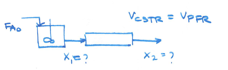
It is proposed to put a CSTR of equal volume upstream of the PFR. Based on the entering molar flow rate to A to the first reactor, what will be the intermediate from the CSTR, X1 , and exit conversion from the PFR, X2 , based on the feed to first reactor?
The entering flow rates and all other variables remain the same as that for the single PFR.
Solution
Gas phase reaction \ce{A -> B}. Isothermal, isobaric PFR
X = 0.632
Base case: PFR
\frac{dX}{dV} = -r_A
-r_A = k C_A
C_A = C_{A0} (1 - X)
\tau k = \int_0^X \frac{1}{1-X} dX
import numpy as np
from scipy.integrate import quad

RHS = lambda x: 1 / (1 - x)
Xf = 0.632
tk, _ = quad(RHS, 0, Xf)
\tau k = 1.00.
CSTR added upstream of PFR. \rightarrow equal volume. Therefore \tau k = 1.00.
V = \frac{F_{A0} X}{k C_{A0} (1-X)} \Rightarrow \tau k = \frac{X}{1 - X}
1 = \frac{X}{1 - X} \Rightarrow X_{1} = 0.5
For X_2
\tau k = \int_{X_1}^{X_2} \frac{dX}{1-X}
This integral can be easily solved by analytical method
1 = \ln \frac{1}{1-X_2} - \ln \frac{1}{1-X_1}
1 - \ln 2 = \ln \frac{1}{1-X_2} \Rightarrow X_2 = 0.82
Here’s alternative numerical way to solve it.
To calculate X_2 from a given X_1 and \tau k, where \tau k is the result of the definite integral from X_1 to X_2 of \frac{dX}{1-X}, you’ll need to perform the inverse operation. Essentially, you need to solve for X_2 in the equation \tau k = \int_{X_1}^{X_2} \frac{dX}{1-X}.
This operation is not straightforward because it requires finding the roots of a function, which is an iterative numerical process. Python’s scipy library has methods such as fsolve for root finding.
import numpy as np
from scipy.integrate import quad
from scipy.optimize import fsolve

def func(x2, x1, tau_k):
    result, _ = quad(lambda x: 1 / (1 - x), x1, x2)
    return result - tau_k

x1 = 0.5
tau_k = 1

# provide a good initial guess for x2
x2_guess = x1 + 0.1

# Solve for x2
x2 = fsolve(func, x2_guess, args=(x1, tau_k))
X_2 = 0.816.
P 5-9
The liquid-phase reaction
\ce{A + B -> C}
follows an elementary rate law and is carried out isothermally in a flow system. The concentrations of the A and B feed streams are 2 M before mixing. The volumetric flow rate of each stream is 5 dm3/min, and the entering temperature is 300 K. The streams are mixed immediately before entering. Two reactors are available. One is a gray, 200.0 dm3 CSTR that can be heated to 77 ^{\circ}C or cooled to 0 ^{\circ}C, and the other is a white, 800.0 dm3 PFR operated at 300 K that cannot be heated or cooled but can be painted red or black. Note that k=0.07 dm^3/mol \cdot min at 300 K and E = 20 kcal/mol.
Which reactor and what conditions do you recommend? Explain the reason for your choice (e.g., color, cost, space available, weather conditions). Back up your reasoning with the appropriate calculations.
How long would it take to achieve 90% conversion in a 200 dm3 batch reactor with CA0 = CB0 = 1 M after mixing at a temperature of 77^{\circ}C?
What would your answer to part (b) be if the reactor were cooled to 0^{\circ}C?
What conversion would be obtained if the CSTR and PFR were operated at 300 K and connected in series? In parallel with 5 mol/min to each?
Keeping Table 1 in mind, what batch reactor volume would be necessary to process the same amount of species A per day as the flow reactors, while achieving 90% conversion?
| C_A=\frac{F_A}{v} = \frac{F_{A0}(1 - X)}{v} | = \frac{F_{A0}(1 - X)}{v_0(1 + eX)}\left(\frac{T_0}{T}\right)\frac{P}{P_0} | = C_{A0} \frac{(1 - X)}{(1 + eX)}\left(\frac{T_0}{T}\right)\frac{P}{P_0} |
| C_B=\frac{F_B}{v} = \frac{F_{A0}(\Theta_B - (b/a)X)}{v} | = \frac{F_{A0}(\Theta_B - (b/a)X)}{v_0(1 + eX)}\left(\frac{T_0}{T}\right)\frac{P}{P_0} | = C_{A0} \frac{(\Theta_B - (b/a)X)}{(1 + eX)}\left(\frac{T_0}{T}\right)\frac{P}{P_0} |
| C_C=\frac{F_C}{v} = \frac{F_{A0}(\Theta_C + (c/a)X)}{v} | = \frac{F_{A0}(\Theta_C + (c/a)X)}{v_0(1 + eX)}\left(\frac{T_0}{T}\right)\frac{P}{P_0} | = C_{A0} \frac{(\Theta_C + (c/a)X)}{(1 + eX)}\left(\frac{T_0}{T}\right)\frac{P}{P_0} |
| C_D=\frac{F_D}{v} = \frac{F_{A0}(\Theta_D + (d/a)X)}{v} | = \frac{F_{A0}(\Theta_D + (d/a)X)}{v_0(1 + eX)}\left(\frac{T_0}{T}\right)\frac{P}{P_0} | = C_{A0} \frac{(\Theta_D + (d/a)X)}{(1 + eX)}\left(\frac{T_0}{T}\right)\frac{P}{P_0} |
| C_1=\frac{F_1}{v} = \frac{F_{A0}\Theta_1}{v} | = \frac{F_{A0}\Theta_1}{v_0(1 + eX)}\left(\frac{T_0}{T}\right)\frac{P}{P_0} | = C_{A0}\Theta_1 \frac{1}{(1 + eX)}\left(\frac{T_0}{T}\right)\frac{P}{P_0} |
Solution
- recommended reactor and conditions
import numpy as np
from scipy.integrate import quad
from scipy.optimize import fsolve

# Data

k_300 = 0.07 # dm^3/mol min
E = 20*1000  # cal/mol
R = 1.987    # cal/mol K

V_CSTR = 200 # dm^3
V_PFR = 800  # dm^3

v_0A = 5     # dm^3/min
v_0B = 5     # dm^3/min

v_0 = v_0A + v_0B

C_Ain = 2    # mol/dm^3
C_Bin = 2    # mol/dm^3

F_A0 = C_Ain * v_0A
F_B0 = C_Bin * v_0B

C_A0 = F_A0/v_0
C_B0 = F_B0/v_0

# Calculate k at 77 degC (350 K)

k_350 = k_300 * np.exp( (E/R) * ((1/300) - (1/350)) )
k_273 = k_300 * np.exp( (E/R) * ((1/300) - (1/273)) )

# CSTR conversion

# Calculate concentrations and rate
CA = lambda x: C_A0 * (1 - x)
CB = lambda x: C_B0 * (1 - x)

rA = lambda x,k: k * CA(x) * CB(x)

# Function to find the root of
def func(x, *args):
    v, fa0, k = args
    rate = rA(x,k)
    return x - v * rate/ fa0

x_guess = 0

x_cstr = fsolve(func, x2_guess, args=(V_CSTR, F_A0, k_350))
X_{CSTR} at 350 K = 0.926.
To calculate the PFR conversion we solve
\frac{dX}{dV} = \frac{-r_A}{F_{A0}}
using similar approach from problem P 5-8.
# PFR conversion

def find_x(x1, *args):
    v, k, fa0 = args
    result, _ = quad(lambda x: 1 / rA(x,k), 0, x1)
    return fa0 * result - v

x_guess = 0
x_pfr = fsolve(find_x, x_guess, args=(V_PFR, k_300, F_A0))
X_{PFR} at 300 K = 0.848.
As the PFR conversion is lower than CSTR conversion, use of CSTR operating at 350 K is recommended.
- Batch time
# Batch time

v = 200 # dm^3
N_A0 = 200  # moles
N_B0 = 200   # moles
X = 0.9

batch_time, _ = quad(lambda x: N_A0 / (rA(x, k_350) * v), 0, X)
Batch time at 350 K = 1.065 min.
- Batch time at 273 K
batch_time, _ = quad(lambda x: N_A0 / (rA(x, k_273) * v), 0, X) Batch time at 273 K = 3550.191 min (2.5 days).
- CSTR / PFR connected in series
# Function to find the root of
def func(x, *args):
    v, fa0, k = args
    rate = rA(x,k)
    return x - v * rate/ fa0

x_guess = 0

x_cstr_1 = fsolve(func, x2_guess, args=(V_CSTR, F_A0, k_300))

def find_x(x2, *args):
    x1, v, k, fa0 = args
    result, _ = quad(lambda x: 1 / rA(x,k), x1, x2)
    return fa0 * result - v

x_guess = x_cstr_1
x_pfr_2 = fsolve(find_x, x_guess, args=(x_cstr_1, V_PFR, k_300, F_A0))
X_{1, CSTR} at 300 K = 0.440.
X_{2, PFR} at 300 K = 0.865.
- CSTR and PFR connected in parallel
# Function to find the root of
def func(x, *args):
    v, fa0, k = args
    rate = rA(x,k)
    return x - v * rate/ fa0

x_guess = 0

x_cstr_1 = fsolve(func, x2_guess, args=(V_CSTR, F_A0/2, k_300))

def find_x(x2, *args):
    x1, v, k, fa0 = args
    result, _ = quad(lambda x: 1 / rA(x,k), x1, x2)
    return fa0 * result - v

x_guess = 0
x_pfr_2 = fsolve(find_x, x_guess, args=(0, V_PFR, k_300, F_A0/2))
X_{1, CSTR} at 300 K = 0.555.
X_{2, PFR} at 300 K = 0.918.
X_{Final} = 0.736.
P 5-11
The irreversible elementary gas-phase reaction
\ce{A + B -> C + D}
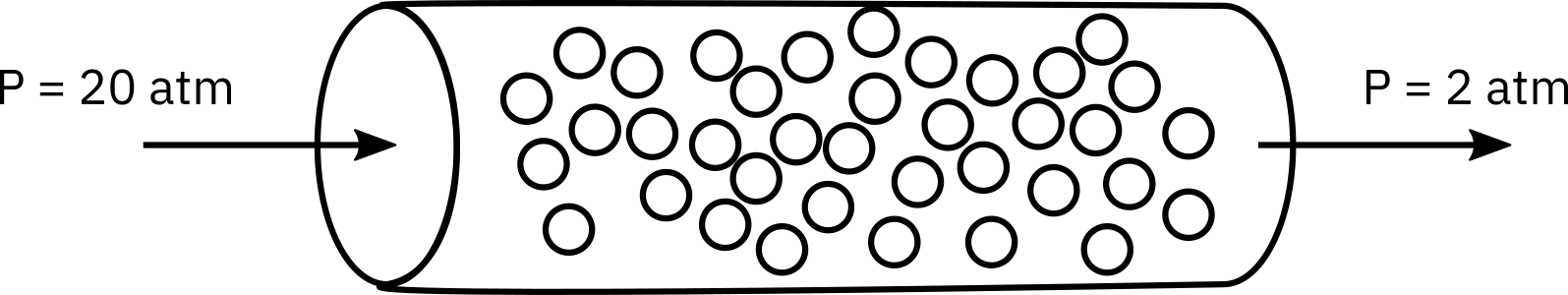
is carried out isothermally at 305 K in a packed-bed reactor with 100 kg of catalyst.
The entering pressure was 20 atm and the exit pressure is 2 atm. The feed is equal molar in A and B and the flow is in the turbulent flow regime, with FA0 = 10 mol/min and CA0 = 0.4 mol/dm3. Currently 80% conversion is achieved. What would be the conversion if the catalyst particle size were doubled and everything else remained the same?
Solution
Elementary reaction
\ce{A + B -> C + D}
From the initial conversion data given, we will determine rate constant. And use this rate constant to calculate coversion when catalyst particle size is dubbled.
Isothermal reaction
C_A = C_{A0}(1-X) \frac{P}{P_0}
let P/P_0 = y. For single isothermal reactions with \epsilon = 0, y^2 = 1 - \alpha w
Equimolar flow of A and B. Therefore, C_A = C_B
-r'_A = k C_A C_B = k C_A^2 = k C_{A0}^2 (1-X)^2 y^2 \tag{1}
\frac{dX}{dW} = \frac{-r'_A}{F_{A0}} \tag{2}
\frac{dy}{dW} = - \frac{\alpha}{2p} \tag{3}
\frac{dX}{dW} = \frac{k C_{A0}^2 (1-X)^2 y^2 }{F_{A0}}
\frac{dX}{(1 - X)^2} = \frac{k C_{A0}^2} {F_{A0}} (1 - \alpha w)^2 dW
\int_0^X \frac{dX}{(1 - X)^2} = \frac{k C_{A0}^2} {F_{A0}} \int_0^W (1 - \alpha w)^2 dW
\frac{X}{(1 - X)} = \frac{k C_{A0}^2} {F_{A0}} \left[ W - \frac{\alpha W^2}{2} \right] \tag{4}
y = 2/20 = 0.1, y^2 = 1 - \alpha W. Therefore, \alpha = (1 - (0.1)^2)/(100) = 9.9 \times 10^{-3} 1/kg
Substituting in Equation 4 we get k = 4.95 dm^6/(kg-cat \ mol \ min).
For Turbulent flow, \alpha \approx 1/Dp. Therefore, as the particle size doubles, \alpha will be halved. \alpha = 4.95 \times 10^{-3}
Substituting in Equation 4: X = 0.86
Alternate approach
We can solve Equation 1, Equation 2, and Equation 3 simultaneously to obtain conversion and pressure as a function of weight.
As we do not know k value, we will use root finding to find the value of k that satisfies the condition where X reaches X_{final} at W_{final}.
import numpy as np
from scipy.integrate import solve_ivp
from scipy.optimize import root_scalar

T = 305 # K
W = 100 # kg
F_A0 = 10 # mol/min
C_A0 = 0.4 # mol/dm^3
X_final = 0.8
P_0 = 20 # atm
P = 2    # atm

# Calculate alpha using pressure drop data

y = P/P_0
alpha_1 = (1 - y**2)/W


# System of differential equations
def system(W, y, *args):
    X, p = y
    k, ca0, fa0, alpha = args

    rate = k * ca0**2 * (1-X)**2 * p**2
    dX_dW = rate / fa0
    dp_dW = -alpha / (2*p)
    return [dX_dW, dp_dW]

# initial conditions
# at start of reactor, conversion is 0 and p is 1
y0 = [0, 1]

# Function to integrate over W
def solve_k(k):
    system_args = (k, C_A0, F_A0, alpha_1)
    sol = solve_ivp(system, [0, W], y0, args=system_args, dense_output=True)
    X = sol.sol(W)[0]
    return X - X_final

# Use root finding to solve for k
# since we don't know the value of k we provide a very large search space

result = root_scalar(solve_k, bracket=[1e-4, 1e4], method='bisect')
k = result.root

# Now alpha is alpha/2
alpha_2 = alpha_1/2

# Calculate the final conversion with this new alpha value
system_args = (k, C_A0, F_A0, alpha_2)
sol = solve_ivp(system, [0, W], y0, args=system_args, dense_output=True)
X = sol.sol(W)[0]
k = 4.963.
X (for \alpha = 0.005) = 0.856.
P 5-24
The gas-phase reaction
\ce{A + B -> C + D}
takes place isothermally at 300 K in a packed-bed reactor in which the feed is equal molar in A and B with CA0 = 0.1 mol/dm3. The reaction is second order in A and zero order in B. Currently, 50% conversion is achieved in a reactor with 100 kg of catalysts for a volumetric flow rate 100 dm3/min. The pressure-drop parameter, \alpha, is \alpha = 0.0099 kg–1. If the activation energy is 10,000 cal/mol, what is the specific reaction rate constant at 400 K?
Solution
import numpy as np
from scipy.integrate import solve_ivp
from scipy.optimize import root_scalar

T = 300 # K
W = 100 # kg
v_0 = 100 # dm^3/min
C_A0 = 0.1 # mol/dm^3
F_A0 = C_A0 * v_0 # mol/min
X_final = 0.5
alpha_1 = 0.0099 # 1/kg

# System of differential equations
def system(W, y, *args):
    X, p = y
    k, ca0, fa0, alpha = args

    rate = k * ca0**2 * (1-X)**2 * p**2
    dX_dW = rate / fa0
    dp_dW = -alpha / (2*p)
    return [dX_dW, dp_dW]

# initial conditions
# at start of reactor, conversion is 0 and p is 1
y0 = [0, 1]

# Function to integrate over W
def solve_k(k):
    system_args = (k, C_A0, F_A0, alpha_1)
    sol = solve_ivp(system, [0, W], y0, args=system_args, dense_output=True)
    X = sol.sol(W)[0]
    return X - X_final

# Use root finding to solve for k
# since we don't know the value of k we provide a very large search space

result = root_scalar(solve_k, bracket=[1e-4, 1e4], method='bisect')
k = result.root

EA = 10000 # cal/mol
T2 = 400
R = 1.987

ln_k2k1 = (EA/R)*((1/T) - (1/T2))

k2 = k*np.exp(ln_k2k1)
k at 300 K = 19.832 dm^6/(kg-cat \ mol \ min).
k at 400 K = 1314.531 dm^6/(kg-cat \ mol \ min).
P 6-4
The elementary gas-phase reaction
\ce{(CH3)3COOC(CH3)3 -> C2H6 + 2 CH3COCH3}
\ce{A -> B + 2 C}
is carried out isothermally at 400 K in a flow reactor with no pressure drop. The specific reaction rate at 50^{\circ}C is 10-4 min-1 (from pericosity data) and the activation energy is 85 kJ/mol. Pure di-tert-butyl peroxide enters the reactor at 10 atm and 127^{\circ}C and a molar flow rate of 2.5 mol/min, i.e., FA = 2.5 mol/min.
Use the algorithm for molar flow rates to formulate and solve the problem. Plot FA, FB, FC, and then X as a function of plug-flow reactor volume and space time to achieve 90% conversion.
Calculate the plug-flow volume and space time for a CSTR for 90% conversion.
Solution
import numpy as np
from scipy.integrate import quad
import matplotlib.pyplot as plt

T_ref = 273.15
R = 0.0821

T0 = 127 + T_ref # K
EA = 85000 # J/mol
P0 = 10 # atm
yA0 = 1

F_A0 = 2.5 # mol/min

C_A0 = yA0 * P0/(R * T0)

delta =  1 + 2 -1
epsilon = yA0 * delta

k_50 = 1e-4 # 1/min
k_127 = k_50* np.exp( (EA/8.314) * (1/(50 + T_ref) - (1/T0)) )

CA = lambda x: C_A0 * (1 - x) / (1 + epsilon * x)
rA = lambda k, x: k * CA(x)

# Molar flow rates
FA = lambda x: F_A0 * (1 - x)
FB = lambda x: F_A0 * (x)
FC = lambda x: F_A0 * (2 * x)

def integral(x, *args):
    fa0, k = args
    return fa0/ rA(k, x)

system_args = (F_A0, k_127)
X_range = np.linspace(0, 0.9, 100)
V = []

# Calculate volume for each X
for X in X_range:
    v, _ = quad(integral, 0, X, args=system_args)
    V.append(v)

plt.plot(V, X_range, label='X vs. Volume')

plt.xlabel('Volume ($dm^3$)')
plt.ylabel('Conversion (X)')
plt.title('Conversion X as a Function of Reactor Volume')

plt.legend()
plt.grid(True)
plt.ylim(0,1)
plt.xlim(0,1000)

plt.show()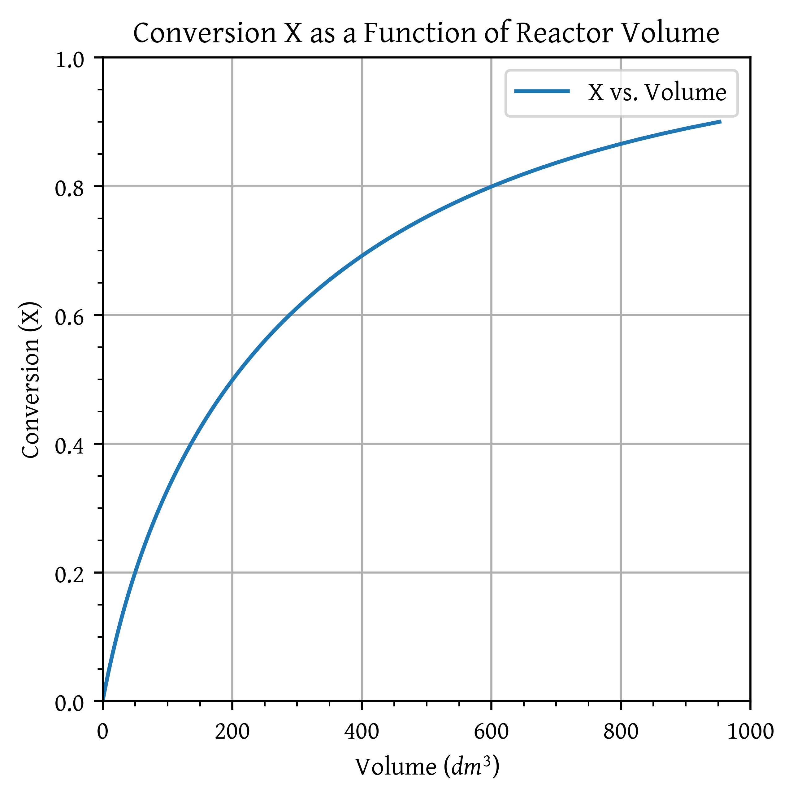
FA_v = FA(X_range)
FB_v = FB(X_range)
FC_v = FC(X_range)

plt.plot(V, FA_v, label='FA')
plt.plot(V, FB_v, label='FB')
plt.plot(V, FC_v, label='FC')

plt.xlabel('Volume ($dm^3$)')
plt.ylabel('Molar Flow Rate (mol/min)')
plt.title('Molar Flow Rates of A, B, and C as Functions of Reactor Volume')

plt.legend()
plt.grid(True)
plt.xlim(0, 1000)

plt.show()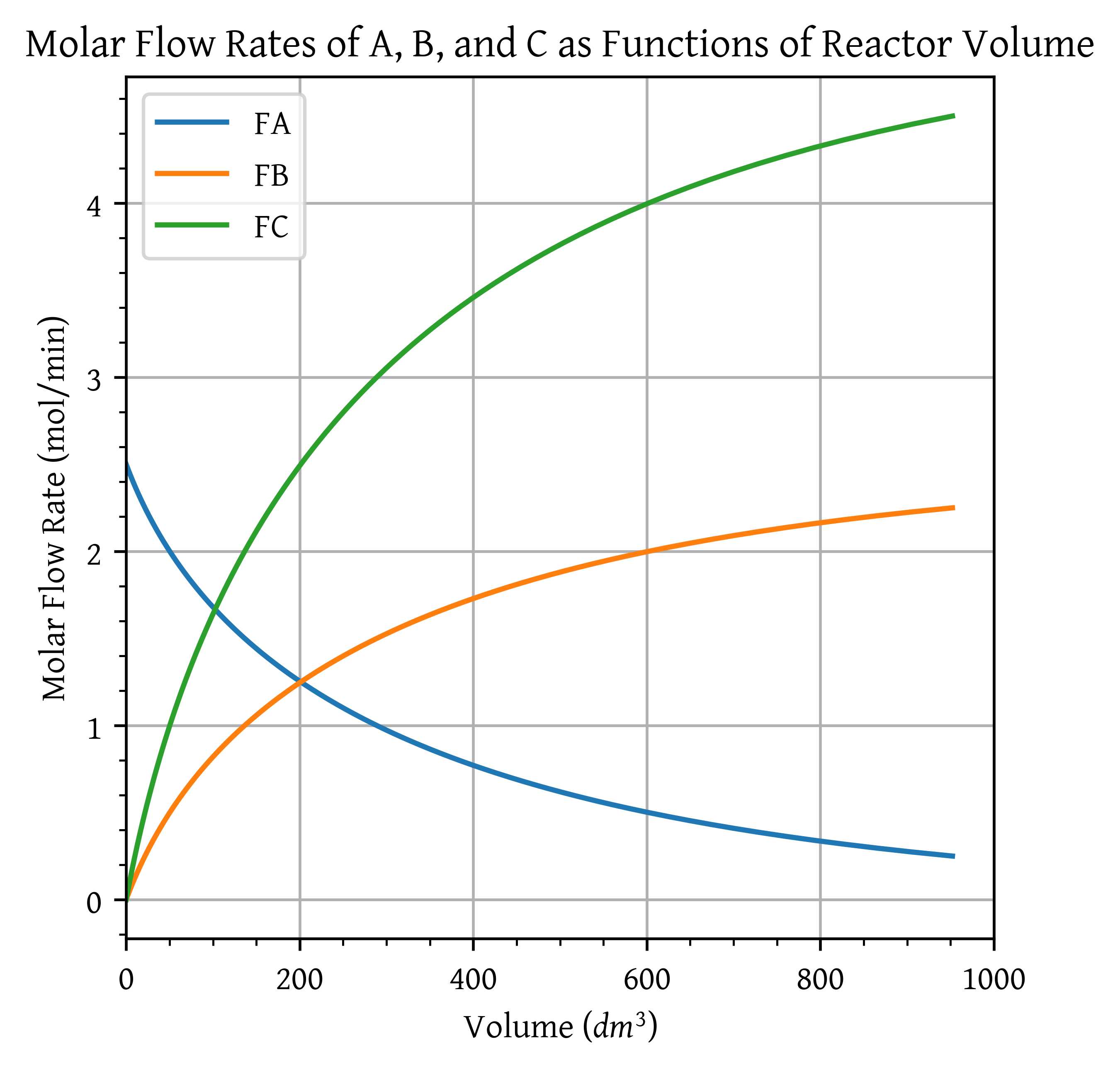
x_final = 0.9

system_args = (F_A0, k_127)
V_PFR, _ = quad(integral, 0, x_final, args=system_args)
V_CSTR = F_A0 * x_final / rA(k_127, x_final)

v0 = F_A0/ C_A0
v = v0 *(1 + epsilon * x_final)
tau = V_CSTR/v
V_{PFR} for X = 0.90 at 127 °C = 952.277 dm^3.
V_{CSTR} for X = 0.90 at 127 °C = 4698.226 dm^3.
\tau_{CSTR} for X = 0.90 at 127 °C = 204.301 min.
P 6-6
(Membrane reactor) The first-order, gas-phase, reversible reaction
\ce{ A <=> B + 2 C }
is taking place in a membrane reactor. Pure A enters the reactor, and B diffuses out through the membrane. Unfortunately, a small amount of the reactant A also diffuses through the membrane.
Plot and analyze the flow rates of A, B, and C and the conversion X down the reactor, as well as the flow rates of A and B through the membrane.
Next, compare the conversion profiles in a conventional PFR with those of a membrane reactor from part (a). What generalizations can you make?
Would the conversion of A be greater or smaller if C were diffusing out instead of B?
Discuss qualitatively how your curves would change if the temperature were increased significantly or decreased significantly for an exothermic reaction. Repeat the discussion for an endothermic reaction.
Additional information:
| k = 10 min-1 | FA0 = 100 mol/min |
| KC = 0.01 mol/dm3 | v_0 = 100 dm3/min |
| kCA= 1 min-1 | Vreactor = 20 dm3 |
| kCB = 40 min-1 |
Solution
import numpy as np
from scipy.integrate import solve_ivp
import matplotlib.pyplot as plt


# Data
k = 10       # 1/min
K_eq = 0.01  # mol/dm^3^
k_CA = 1     # min^-1^
k_CB = 40    # min^-1^

F_A0 =  100    # mol/min
v_0  = 100     # dm^3^/min
V_reactor = 20 # dm^3^

C_T0 = F_A0/v_0

r_A = lambda ca, cb, cc: - k * (ca - cb * cc**2/ K_eq )
r_B = lambda ca, cb, cc: - r_A(ca, cb, cc)
r_C = lambda ca, cb, cc: - r_A(ca, cb, cc)/2

r_diff_A = lambda ca: k_CA * ca
r_diff_B = lambda cb: k_CB * cb

C = lambda f, ft: C_T0 * f/ft

# System of differential equations for membrane reactor
def membrane_reactor(V, y, *args):
    FA, FB, FC = y

    FT = FA + FB + FC
    CA = C(FA, FT)
    CB = C(FB, FT)
    CC = C(FC, FT)

    dFA_dV = r_A(CA, CB, CC) - r_diff_A(CA)
    dFB_dV = r_B(CA, CB, CC) - r_diff_B(CB)
    dFC_dV = r_C(CA, CB, CC)

    return [dFA_dV, dFB_dV, dFC_dV]

# System of differential equations for pfr
def pfr(V, y, *args):
    FA, FB, FC = y

    FT = FA + FB + FC
    CA = C(FA, FT)
    CB = C(FB, FT)
    CC = C(FC, FT)

    dFA_dV = r_A(CA, CB, CC)
    dFB_dV = r_B(CA, CB, CC)
    dFC_dV = r_C(CA, CB, CC)

    return [dFA_dV, dFB_dV, dFC_dV]

# initial conditions
# at start of reactor, conversion is 0 and p is 1
y0 = [F_A0, 0, 0]

sol_membrane = solve_ivp(membrane_reactor, [0, V_reactor], y0, dense_output=True)
sol_pfr = solve_ivp(pfr, [0, V_reactor], y0, dense_output=True)

# Generating data for plotting
V = np.linspace(0, V_reactor, 100)
FA_m, FB_m, FC_m = sol_membrane.sol(V)
FA_p, FB_p, FC_p = sol_pfr.sol(V)

# Plotting
plt.plot(V, FA_m, 'b', label='$F_Am$')
plt.plot(V, FB_m, 'g', label='$F_Bm$')
plt.plot(V, FC_m, 'r', label='$F_Cm$')

plt.plot(V, FA_p, 'b--', label='$F_Ap$')
plt.plot(V, FB_p, 'g--', label='$F_Bp$')
plt.plot(V, FC_p, 'r--', label='$F_Cp$')


plt.xlabel('Volume (dm$^3$)')
plt.ylabel('Molar Flow Rate (mol/min)')
plt.title('Molar Flow Rates of A, B, and C in the Reactor')

plt.legend()
plt.grid(True)
plt.xlim(0, 20)

plt.show()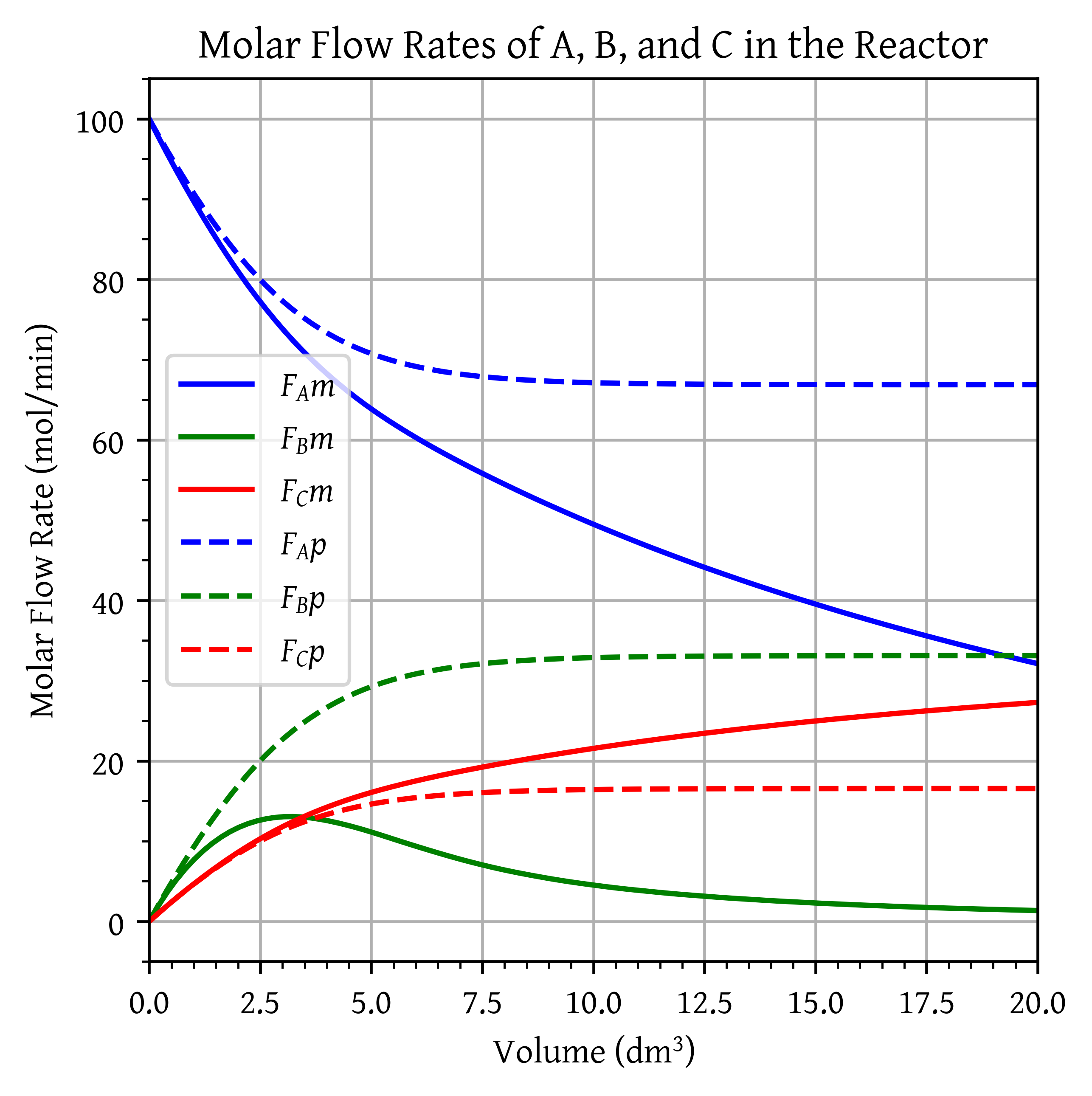
P 6-7
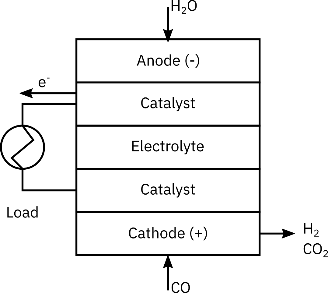
Fuel Cells Rationale. With the focus on alternative clean-energy sources, we are moving toward an increased use of fuel cells to operate appliances ranging from computers to automobiles. For example, the hydrogen/oxygen fuel cell produces clean energy as the products are water and electricity, which may lead to a hydrogen-based economy instead of a petroleum-based economy. A large component in the processing train for fuel cells is the water-gas shift membrane reactor. (M. Gummala, N. Gupla, B. Olsomer, and Z. Dardas, Paper 103c, 2003, AIChE National Meeting, New Orleans, LA.)
\ce{CO + H2O <=> CO2 + H2}
Here, CO and water are fed to the membrane reactor containing the catalyst. Hydrogen can diffuse out the sides of the membrane, while \ce{CO}, \ce{H2O}, and \ce{CO2} cannot. Based on the following information, plot the concentrations and molar flow rates of each of the reacting species down the length of the membrane reactor.
Assume the following: The volumetric feed is 10 dm3/min at 10 atm, and the equimolar feed of CO and water vapor with CT0 = 0.4 mol/dm3. The equilibrium constant is Ke = 1.44, with k = 1.37 dm^6/ \text{mol kg-cat} \cdot \text{min}, and the mass transfer coefficient k_{H_2} = 0.1 dm^3/ \text{kg-cat} \cdot \text{min}
(Hint: First calculate the entering molar flow rate of CO and then relate FA and X.)
What is the membrane reactor volume necessary to achieve 85% conversion of CO?
Sophia wants you to compare the MR with a conventional PFR. What will you tell her?
For that same membrane reactor volume, Nicolas wants to know what would be the conversion of CO if the feed rate were doubled?
Solution
import numpy as np
from scipy.integrate import solve_ivp
from scipy.optimize import root_scalar
import matplotlib.pyplot as plt


# Data
k = 1.37
K_eq = 1.44
k_H2 = 0.1

v_0  = 10
p = 10
C_T0 = 0.4

F_A0 = C_T0* v_0/2
F_B0 = C_T0* v_0/2
F_C0 = 0
F_D0 = 0


# A, B, C, D --> CO, H2O, CO2, H2

# System of differential equations for membrane reactor
def fuel_cell(V, y, *args):
    FA, FB, FC, FD = y

    FT = FA + FB + FC + FD

    CA = C_T0 * FA / FT
    CB = C_T0 * FB / FT
    CC = C_T0 * FC / FT
    CD = C_T0 * FD / FT

    rate = -k * (CA * CB - CC * CD/ K_eq)

    rA = rate
    rB = rate
    rC = -rate
    rD = -rate

    rH2 = k_H2 * CD

    dFA_dV = rA
    dFB_dV = rB
    dFC_dV = rC
    dFD_dV = rD - rH2

    return [dFA_dV, dFB_dV, dFC_dV, dFD_dV]

# initial conditions
# at start of reactor, conversion is 0 and p is 1
y0 = [F_A0, F_B0, F_C0, F_D0]

V_reactor = 500
sol_fuel_cell = solve_ivp(fuel_cell, [0, V_reactor], y0, dense_output=True)


def target(V):
    FA = sol_fuel_cell.sol(V)[0]  # Get FA at V
    return FA - F_A0*(1-0.85)

result = root_scalar(target, bracket=[0, V_reactor], method='bisect')
v_x85 =  result.root


# Generating data for plotting
V = np.linspace(0, V_reactor, 100)
FA, FB, FC, FD = sol_fuel_cell.sol(V)

# Plotting
plt.plot(V, FA, 'b', label='$F_A$')
plt.plot(V, FB, 'g', label='$F_B$')
plt.plot(V, FC, 'r', label='$F_C$')
plt.plot(V, FD, 'm', label='$F_D$')

plt.xlabel('Volume (dm$^3$)')
plt.ylabel('Molar Flow Rate (mol/min)')
plt.title('Molar Flow Rates of A, B, C, and D in the Reactor')

plt.legend()
plt.grid(True)
plt.xlim(0, V_reactor)

plt.show()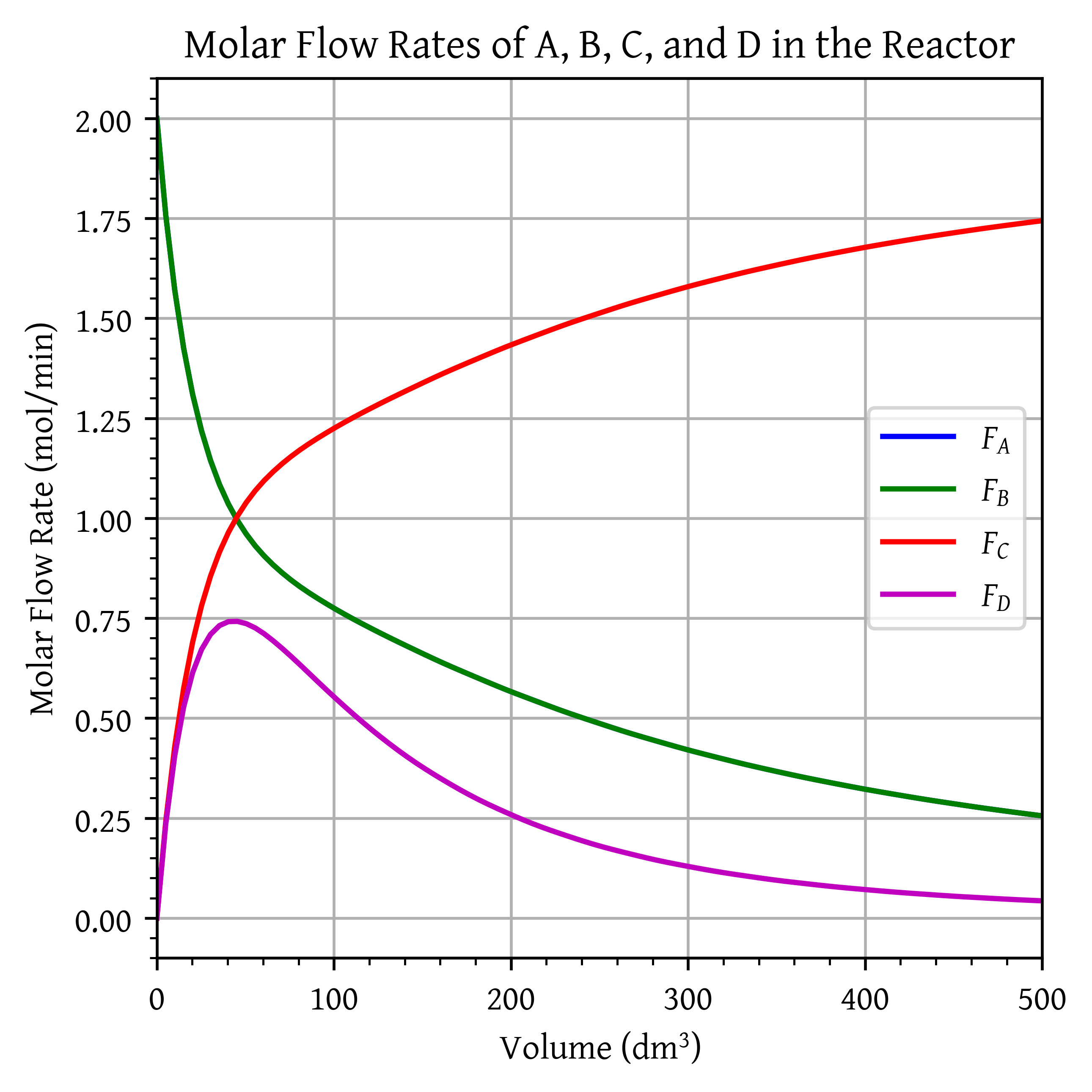
Volume of reacctor to achieve X = 0.85: 429.53 dm^3.
References
Fogler, H. Scott. 2016. Elements of Chemical Reaction Engineering. Fifth edition. Boston: Prentice Hall.
Citation
BibTeX citation:
@online{utikar2024,
  author = {Utikar, Ranjeet},
  title = {Solutions to Workshop 04: {Isothermal} Reactor Design},
  date = {2024-03-19},
  url = {https://cre.smilelab.dev/content/workshops/04-isothermal-reactor-design/solutions.html},
  langid = {en}
}
For attribution, please cite this work as:
Utikar, Ranjeet. 2024. “Solutions to Workshop 04: Isothermal
Reactor Design.” March 19, 2024. https://cre.smilelab.dev/content/workshops/04-isothermal-reactor-design/solutions.html.