Solutions to workshop 11: Distribution of residence time

Lecture notes for chemical reaction engineering

Try following problems from Fogler 5e (Fogler (2016)) P 16-3, P 16-6, P 16-11

We will go through some of these problems in the workshop.

P 16-3

Consider the E(t) curve below.

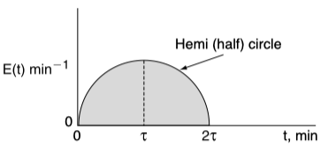
Mathematically this hemi circle is described by these equations:

For 2\tau >= t >= 0, then E(t) = \sqrt{\tau^2 - (t - \tau)^2} min^–1 (hemi circle)

For t > 2\tau, then E(t) = 0

1. What is the mean residence time?

2. What is the variance?

Solution

Hand written solution

import sympy as sp
from IPython.display import display, Markdown

# Define variables
t, u= sp.symbols('t, u')
tau = sp.symbols('tau', real=True, positive=True)

et = sp.sqrt(tau**2 - (t - tau)**2)
# using u = t - tau integral becomes
# E(t) = int from -tau to tau ( sqrt (tau^2 - u^2))
integral_eu = sp.integrate(sp.sqrt(tau**2 - u**2), (u, -tau, tau))

tau_est = sp.solve(integral_eu - 1, tau)

# Evaluate the numeric value of tau_est
tau_numeric = tau_est[0].evalf()

Integral of E(t):

integral_latex = sp.latex(integral_eu)
display(Markdown(f"$$E(t) = {integral_latex}$$"))

E(t) = \frac{\pi \tau^{2}}{2}

Solution for \tau

tau_latex = sp.latex(sp.simplify(tau_est[0]))
display(Markdown(f"$$\\tau = {tau_latex}$$"))

\tau = \frac{\sqrt{2}}{\sqrt{\pi}}

\tau = 0.798 min.

We can also solve this problem numerically

import numpy as np
from scipy.integrate import quad
from scipy.optimize import fsolve
from IPython.display import display, Markdown

# Define E(t) function
def et(t, tau):
    if 0 <= t <= 2 * tau:
        return np.sqrt(tau**2 - (t - tau)**2)
    else:
        return 0

# Function to find tau such that the integral equals 1
def integral(tau):
    res, _ = quad(et, 0, 2 * tau, args=(tau,))
    return res - 1

# Initial guess for tau
tau_guess = 1

# Solve for tau
tau_est = fsolve(integral, tau_guess)[0]

# Define the variance function
def variance_func(t, tau):
    return (t - tau)**2 * et(t, tau)

# Calculate the variance using numerical integration
variance_value, _ = quad(variance_func, 0, 2 * tau_est, args=(tau_est,))

Using numerical method:

\tau \approx 0.798 min.

\sigma^2 \approx 0.159 min².

P 16-6

An RTD experiment was carried out in a nonideal reactor that gave the following results:

E(t) = 0	for	t < 1 \, min
E(t) = 1.0 \, min^{-1}	for	1 <= t <= 2 \, min
E(t) = 0	for	t > 2 \, min

1. What are the mean residence time, t_m, and variance \sigma^2?

2. What is the fraction of the fluid that spends a time 1.5 minutes or longer in the reactor?

3. What fraction of fluid spends 2 minutes or less in the reactor?

4. What fraction of fluid spends between 1.5 and 2 minutes in the reactor?

Solution

Hand written solution, (Accompanying excel file).

import numpy as np
from scipy.integrate import quad
from IPython.display import display, Markdown

# Define E(t) function
def et(t):
    if t < 1:
        return 0
    elif 1 <= t <= 2:
        return 1.0
    else:
        return 0

# Mean residence time function
def tau_func(t):
    return t * et(t)

# Variance function
def variance_func(t, tm):
    return (t - tm)**2 * et(t)

# Calculate mean residence time (t_m)
tau, _ = quad(tau_func, 0, np.inf)

# Calculate variance (sigma^2)
variance, _ = quad(variance_func, 0, np.inf, args=(tau,))

# Fraction of fluid that spends 1.5 minutes or longer
f1_5_inf, _ = quad(et, 1.5, np.inf)

# Fraction of fluid that spends 2 minutes or less
f0_2, _ = quad(et, 0, 2)

# Fraction of fluid that spends between 1.5 and 2 minutes
f1_5_2, _ = quad(et, 1.5, 2)

Mean Residence Time \tau \approx 1.5000 min.

Variance \sigma^2 \approx 0.0833 min^2.

Fraction of fluid that spends 1.5 minutes or longer: 0.50

Fraction of fluid that spends 2 minutes or less: 1.00

Fraction of fluid that spends between 1.5 and 2 minutes: 0.50

P 16-11

The volumetric flow rate through a reactor is 10 dm³/min. A pulse test gave the following concentration measurements at the outlet:

t (min)	c \times 10^5	t (min)	c \times 10^5
0	0	15	238
0.4	329	20	136
1.0	622	25	77
2	812	30	44
3	831	35	25
4	785	40	14
5	720	45	8
6	650	50	5
8	523	60	1
10	418

1. Plot the external-age distribution E(t) as a function of time.

2. Plot the external-age cumulative distribution F(t) as a function of time.

3. What are the mean residence time t_m and the variance, \sigma^2 ?

4. What fraction of the material spends between 2 and 4 minutes in the reactor?

5. What fraction of the material spends longer than 6 minutes in the reactor?

6. What fraction of the material spends less than 3 minutes in the reactor?

7. Plot the normalized distributions E(\Phi) and F(\Phi) as a function of (\Phi).

8. What is the reactor volume?

9. Plot the internal-age distribution I(t) as a function of time.

10. What is the mean internal age \alpha_m ?

Solution

Hand written solution, (Accompanying excel file).

import numpy as np
from scipy.integrate import quad
from scipy.interpolate import interp1d
import matplotlib.pyplot as plt
from IPython.display import display, Markdown

# Given data
t = np.array([0, 0.4, 1.0, 2.0, 3.0, 4.0, 5.0, 6.0, 
              8.0, 10.0, 15, 20, 25, 30, 35, 40, 45, 50, 60])
c = np.array([0, 329, 622, 812, 831, 785, 720, 650, 
              523, 418, 238, 136, 77, 44, 25, 14, 8, 5, 1]) * 1e-5

# Flow rate
Q = 10  # dm^3/min

# Normalize concentration to calculate E(t)
integral_c = np.trapz(c, t)
et = c / integral_c

# Interpolation functions
et_interp = interp1d(t, et, kind='cubic', fill_value="extrapolate")

# f_interp = lambda t: np.array([quad(et_interp, 0, ti)[0] for ti in t])

# Define cumulative distribution F(t)
def f_interp(t):
    return np.array([quad(et_interp, 0, ti, limit=1000)[0] for ti in np.atleast_1d(t)])

# Mean residence time function
tau_func = lambda t: t * et_interp(t)

# Variance function
variance_func = lambda t, tm: (t - tm)**2 * et_interp(t)

# Calculate mean residence time (t_m)
tau, _ = quad(tau_func, 0, np.max(t))

# Calculate variance (σ²)
variance, _ = quad(variance_func, 0, np.max(t), args=(tau,))

# Plot E(t) and F(t)
t_plot = np.linspace(0, 60, 500)
et_plot = et_interp(t_plot)
f_plot = f_interp(t_plot)

plt.scatter(t, et, label='E(t) experimental')
plt.plot(t_plot, et_plot, label='E(t) fitted')
plt.xlabel('Time (min)')
plt.ylabel('E(t)')
plt.xlim(np.min(t_plot), np.max(t_plot))
plt.ylim(0,0.1)
plt.legend()
plt.show()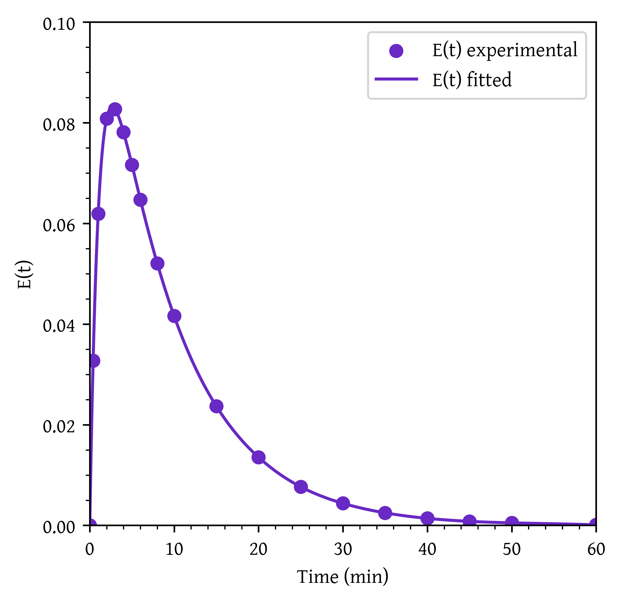

Figure 1: Exit age distribution E(t)

plt.plot(t_plot, f_plot, label='F(t)')
plt.xlabel('Time (min)')
plt.ylabel('F(t)')
plt.xlim(np.min(t_plot), np.max(t_plot))
plt.ylim(0,1)
plt.legend()
plt.show()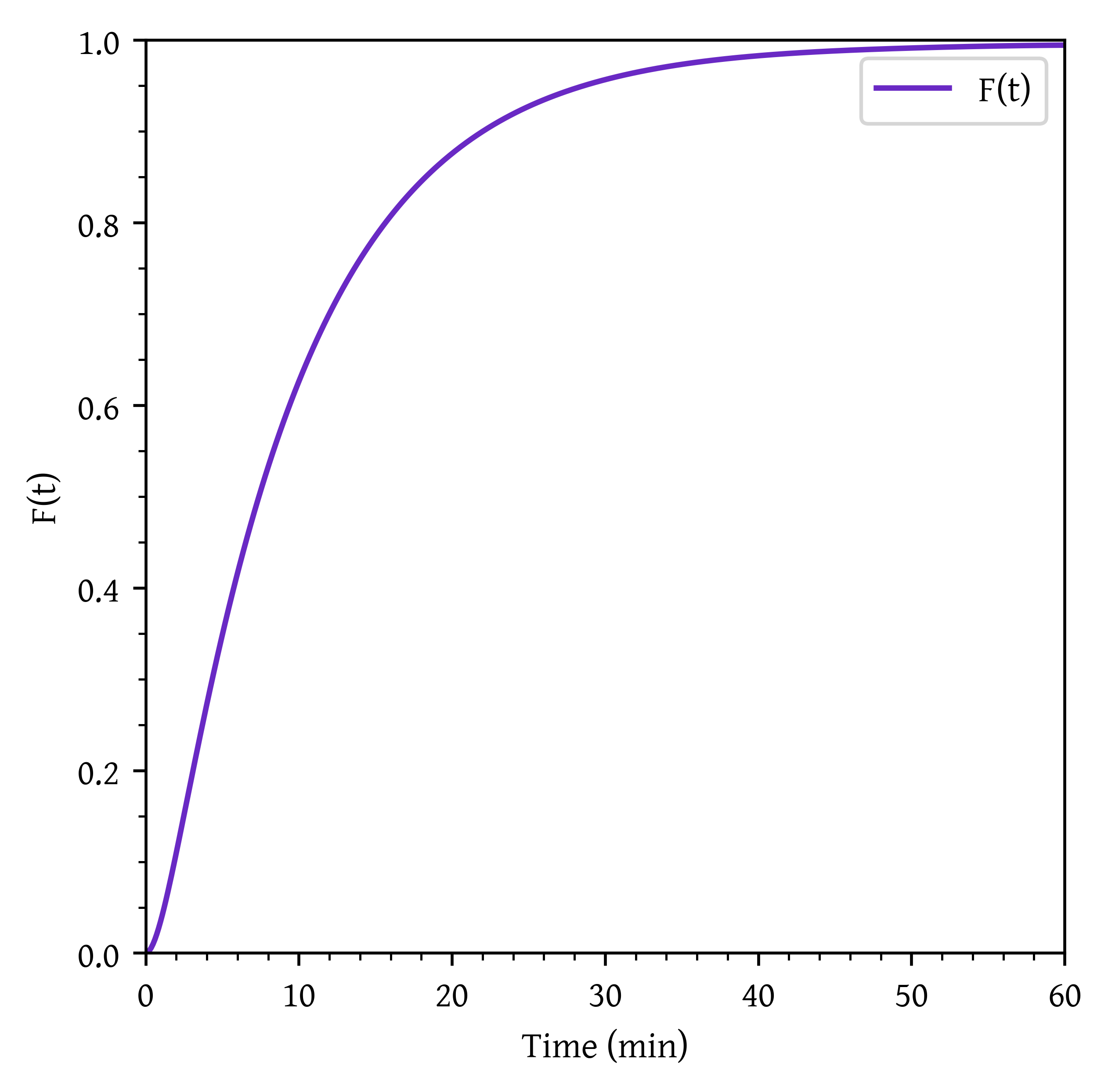

Figure 2: Cumulative distribution F(t)

# Calculate specific time fractions
fraction_2_to_4, _ = quad(et_interp, 2, 4)
fraction_above_6, _ = quad(et_interp, 6, np.max(t))
fraction_below_3, _ = quad(et_interp, 0, 3)

# Reactor volume calculation
volume = Q * tau

Mean Residence Time tau: \approx 9.88 min.

Variance \sigma^2: \approx 75.69 min^2

Specific Time Fractions:

Fraction of material that spends between 2 and 4 minutes: \approx 0.163

Fraction of material that spends longer than 6 minutes: \approx 0.578

Fraction of material that spends less than 3 minutes: \approx 0.193

Reactor Volume: V = Q \cdot \tau: \approx 98.83 dm^3

Normalized distrubution:

To calculate normalized RTD, we convert t to \Theta as \Theta = t/\tau.

The dimensionless RTD function is calculated as E (\Theta) = \tau E(t).

Normalized cumulative RTD: F(\Theta) = \int_0^\Theta E(\Theta)d\Theta

theta = t/tau
e_theta = tau * et
e_theta_interp = interp1d(theta, e_theta, kind='cubic', fill_value="extrapolate")

theta_plot = np.linspace(0, theta[-1], 500)
e_theta_plot = e_theta_interp(theta_plot)

plt.scatter(theta, e_theta, label='$E(\\Theta)$ experimental')
plt.plot(theta_plot, e_theta_plot, label='$E(\\Theta)$ fitted')
plt.xlabel('$\\Theta$')
plt.ylabel('$E(\\Theta)$')
plt.xlim(np.min(theta_plot), np.max(theta_plot))
plt.ylim(0,1)
plt.legend()
plt.show()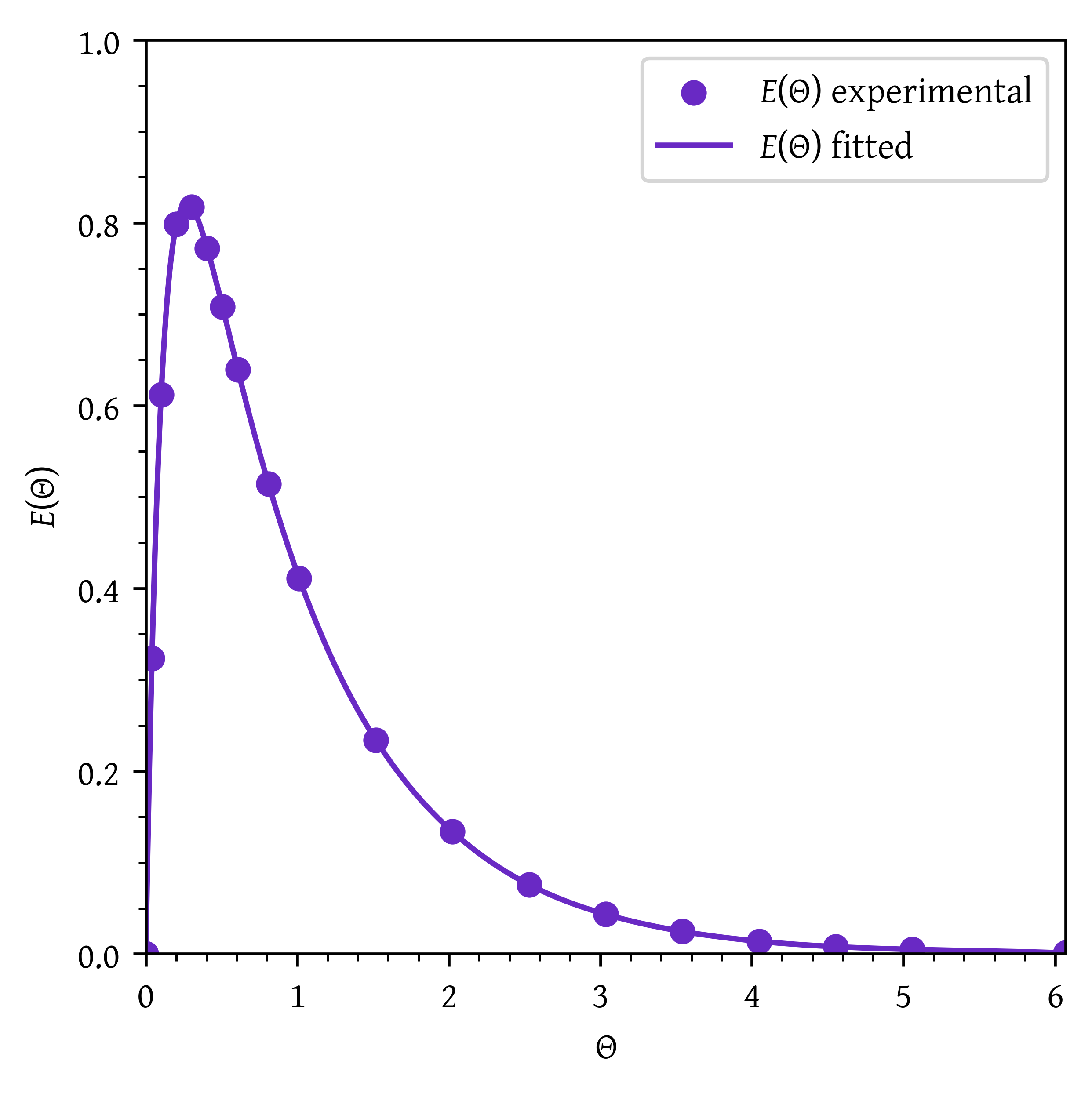

Figure 3: Normalized exit age distribution E(\Theta)

f_theta_interp = lambda t: np.array([quad(e_theta_interp, 0, ti)[0] for ti in t])
f_theta_plot = f_theta_interp(theta_plot)

plt.plot(theta_plot, f_theta_plot, label='$F(\\Theta)$')
plt.xlabel('$\\Theta$')
plt.ylabel('F(t)')
plt.xlim(np.min(theta_plot), np.max(theta_plot))
plt.ylim(0,1)
plt.legend()
plt.show()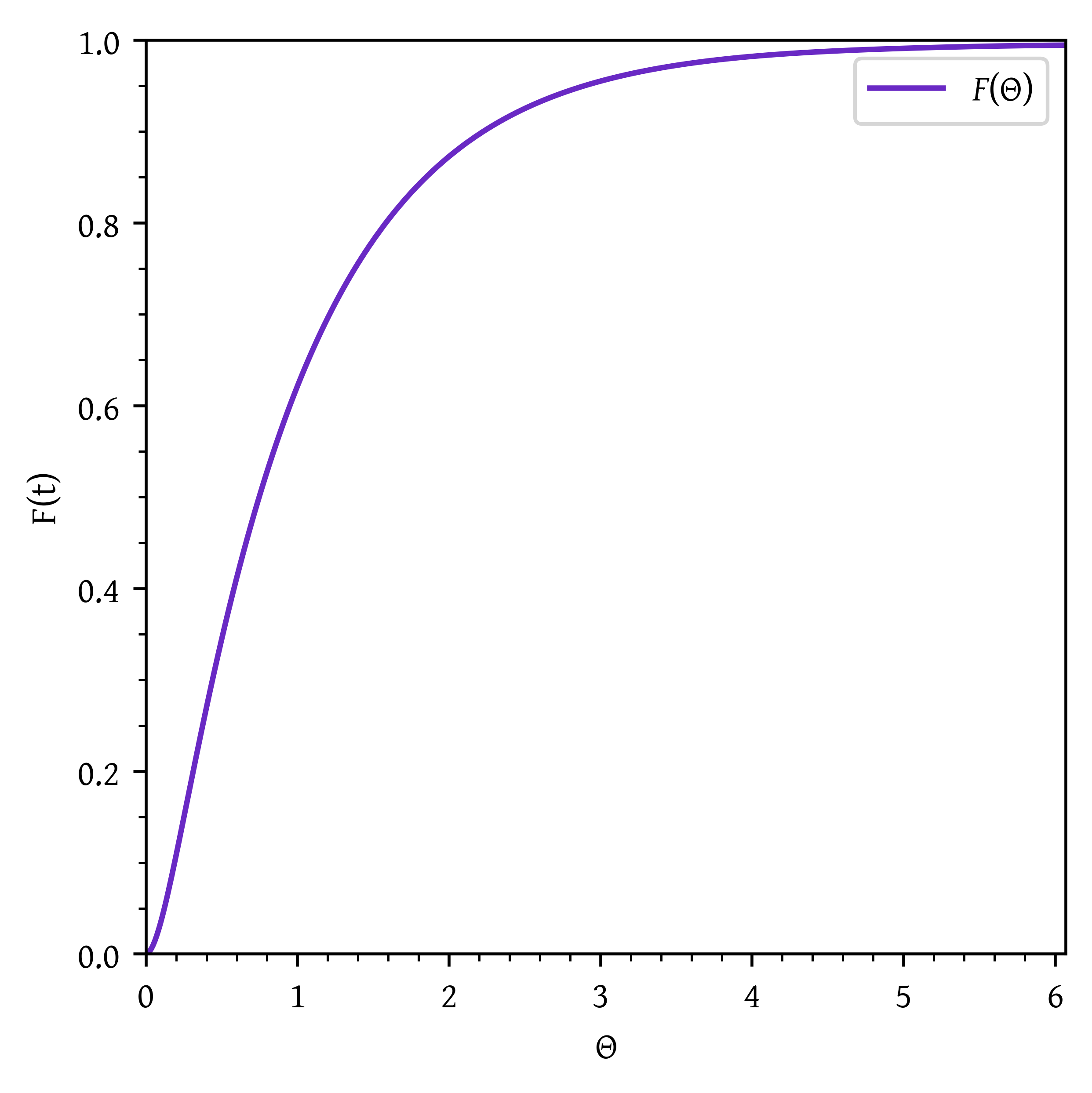

Figure 4: Normalized cumulative distribution F(\Theta)

Internal age distribution

I(t) = \frac{1}{\tau} \left[ 1 - F(t) \right]

Mean internal age

\alpha_m = \int_0^\infty I(t)dt

internal_age = lambda t, tm: (1/tm) * (1 - f_interp(t)) 
mean_internal_age, _ = quad(lambda t: internal_age(t, tau), 0, np.max(t))

it_plot = internal_age(t_plot, tau)

plt.plot(t_plot, it_plot, label='I(t)')
plt.xlabel('Time (min)')
plt.ylabel('I(t)')
plt.xlim(np.min(t_plot), np.max(t_plot))
plt.ylim(0,0.1)
plt.legend()
plt.show()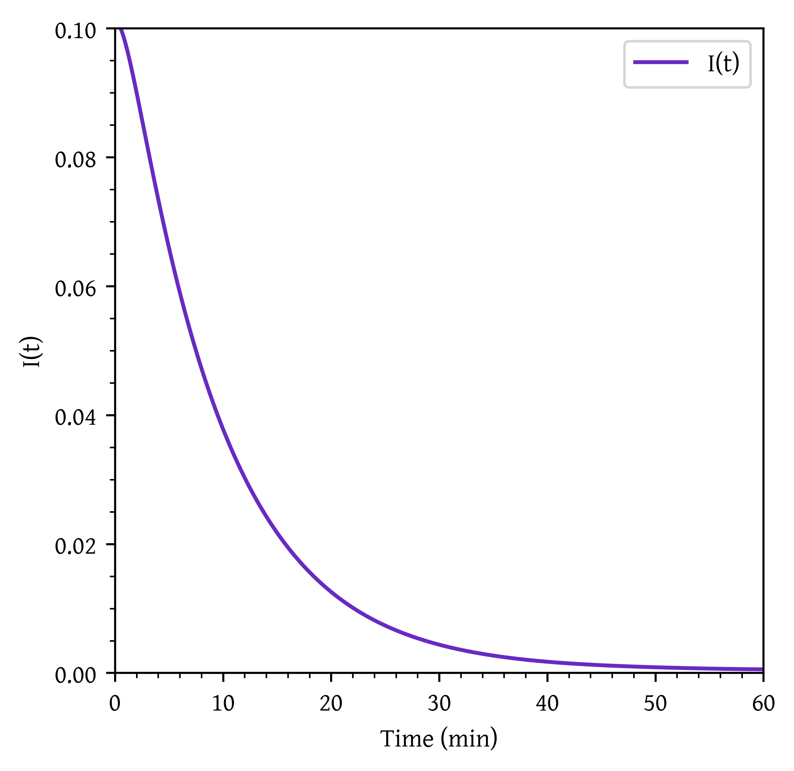

Figure 5: Internal age distribution I(t)

Mean Internal age \alpha_m: \approx 1.03 min.

References

Fogler, H. Scott. 2016. Elements of Chemical Reaction Engineering. Fifth edition. Boston: Prentice Hall.