Solutions to workshop 05: Collection and analysis of rate data

Lecture notes for chemical reaction engineering

Try following problems from Fogler 5e (Fogler 2016). P 7-4, P 7-5, P 7-6, P 7-7, P 7-10

We will go through some of these problems in the workshop.

P 7-4

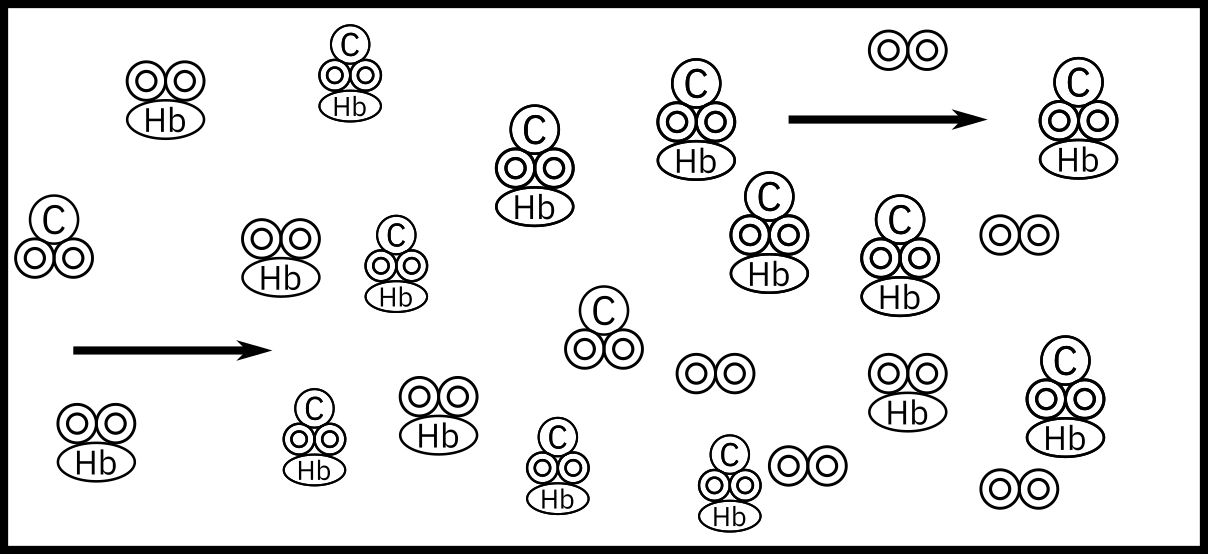
When arterial blood enters a tissue capillary, it exchanges oxygen and carbon dioxide with its environment, as shown in this diagram.

The kinetics of this deoxygenation of hemoglobin in blood was studied with the aid of a tubular reactor by Nakamura and Staub (J. Physiol., 173, 161).

\ce{HbO2 <=>[ $k_1$ ][ $k_{-1}$ ] Hb + O2}

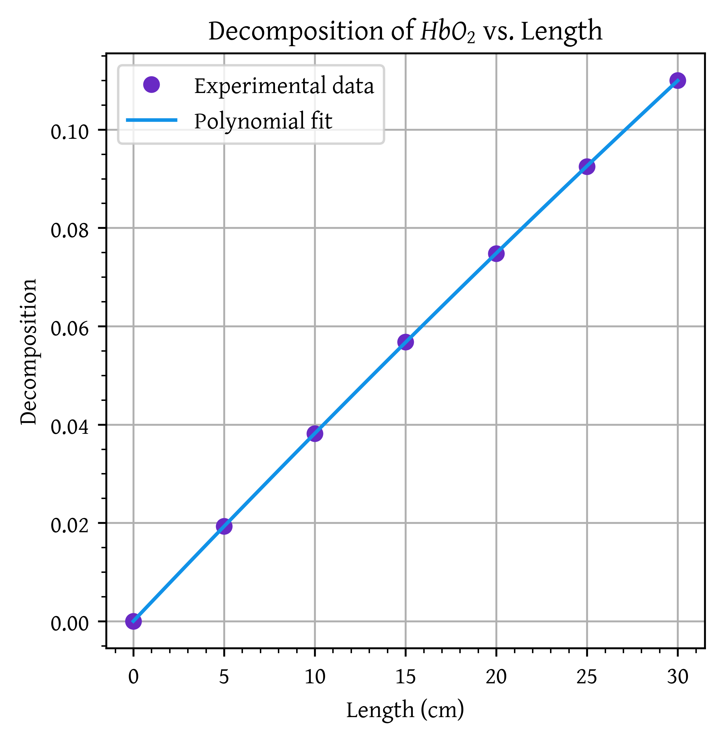
Although this is a reversible reaction, measurements were made in the initial phases of the decomposition so that the reverse reaction could be neglected. Consider a system similar to the one used by Nakamura and Staub: the solution enters a tubular reactor (0.158 cm in diameter) that has oxygen electrodes placed at 5-cm intervals down the tube. The solution flow rate into the reactor is 19.6 cm³/s with C_A0 = 2.33 × 10^–6 mol/cm³.

Electrode position	1	2	3	4	5	6	7
Percent decomposition of \ce{HbO2}	0.00	1.93	3.82	5.68	7.48	9.25	11.00

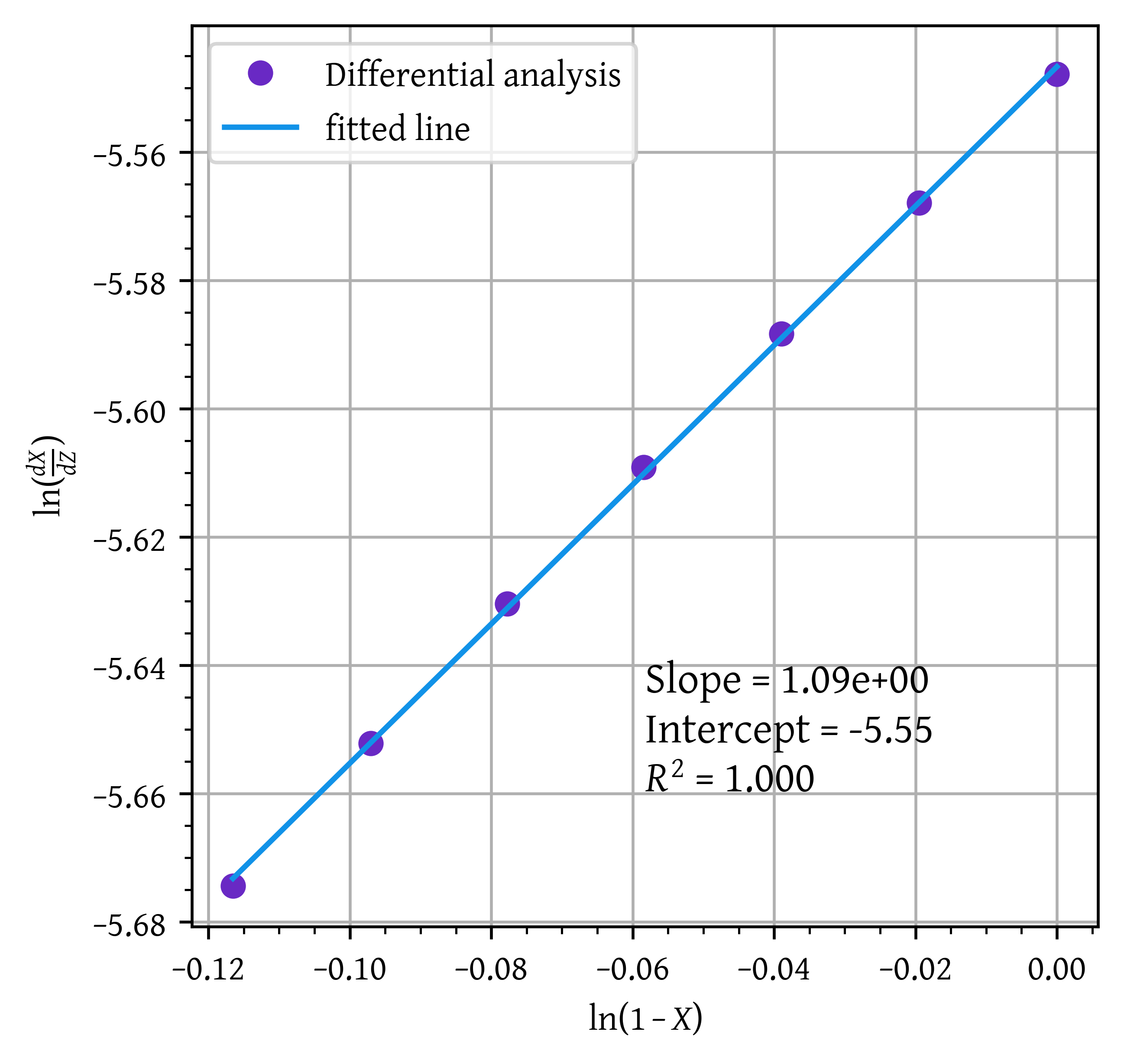
1. Using the method of differential analysis of rate data, determine the reaction order and the forward specific reaction-rate constant k₁ for the deoxygenation of hemoglobin.

2. Repeat using regression.

Solution

• Reaction is reversible, but the measurements were taken in the initial phases where the reverse reaction can be neglected

\ce{HbO2 ->[k] Hb + O2}

• % decomposition (conversion) along the length of PFR is given

Rate law: -r_A = k C_A^\alpha = k C_{A0}^\alpha (1 - X)^\alpha

For PFR: F_{A0}\frac{dX}{dV} = k C_{A0}^\alpha (1 - X)^\alpha

V = A_c Z; \Rightarrow dV = A_c dZ

\frac{dX}{dZ} = \underbrace{ \frac{k C_{A0}^\alpha A_c}{F_{A0}} }_a (1 - X)^\alpha

\frac{dX}{dZ} = a (1 - X)^\alpha

Taking log

\ln \frac{dX}{dZ} = \ln a + \alpha \ln (1 - X)

A plot of \ln \frac{dX}{dZ} vs \ln (1 - X) has a slope of \alpha

import numpy as np
from scipy.stats import linregress
import matplotlib.pyplot as plt

# Data
delta_Z = 5 # cm
C_A0 = 2.33e-6  # mol/cm^3
v_0 = 19.6 # cm^3/s
diameter = 0.158  # cm

Ac = np.pi * diameter**2/4
F_A0 = C_A0 * v_0

electrode_positions = np.array([1, 2, 3, 4, 5, 6, 7])
percent_decomposition = np.array([0, 1.93, 3.82, 5.68, 7.48, 9.25, 11.00])

Z = (electrode_positions - 1) *delta_Z
X = percent_decomposition/100

# fit polynomial to the data
coefficients = np.polyfit(Z, X, deg=2)
polynomial = np.poly1d(coefficients)

z_fit = np.linspace(Z.min(), Z.max(), 100)
x_fit = polynomial(z_fit)

plt.plot(Z, X, 'o', label='Experimental data')
plt.plot(z_fit, x_fit , '-', label='Polynomial fit')
plt.xlabel('Length (cm)')
plt.ylabel('Decomposition')
plt.title('Decomposition of $HbO_2$ vs. Length')

plt.legend()
plt.grid(True)

plt.show()

# calculate the derivative of the polynomial
dxdz = np.polyder(polynomial)

# calculate ln(1-X) and ln(dxdz) --> ideally should do this with fitted data
# ln_1_minus_x = np.log(1-x_fit)
# ln_dxdz = np.log(dxdz(z_fit))

ln_1_minus_x = np.log(1-X)
ln_dxdz = np.log(dxdz(Z))

# fit line
res = linregress(ln_1_minus_x, ln_dxdz)
line = res.slope * ln_1_minus_x + res.intercept

plt.plot(ln_1_minus_x, ln_dxdz, 'o', label='Differential analysis')
plt.plot(ln_1_minus_x, line, '-', label='fitted line')

plt.annotate(
  f'Slope = {res.slope:.2e}\nIntercept = {res.intercept:.2f}\n$R^2$ = {res.rvalue**2:.3f}',
  xy=(0.5, 0.15),
  xycoords='axes fraction',
  fontsize=12
)

plt.xlabel('$\ln (1-X)$')
plt.ylabel('$\ln(\\frac{dX}{dZ})$')

plt.legend()
plt.grid(True)

plt.show()

# pick the closest round order
order = round(res.slope)
a = np.exp(res.intercept)
k = a * F_A0 / (C_A0**order * Ac)

Reaction order is = 1, and k is 3.899 1/s.

P 7-5

The liquid-phase irreversible reaction

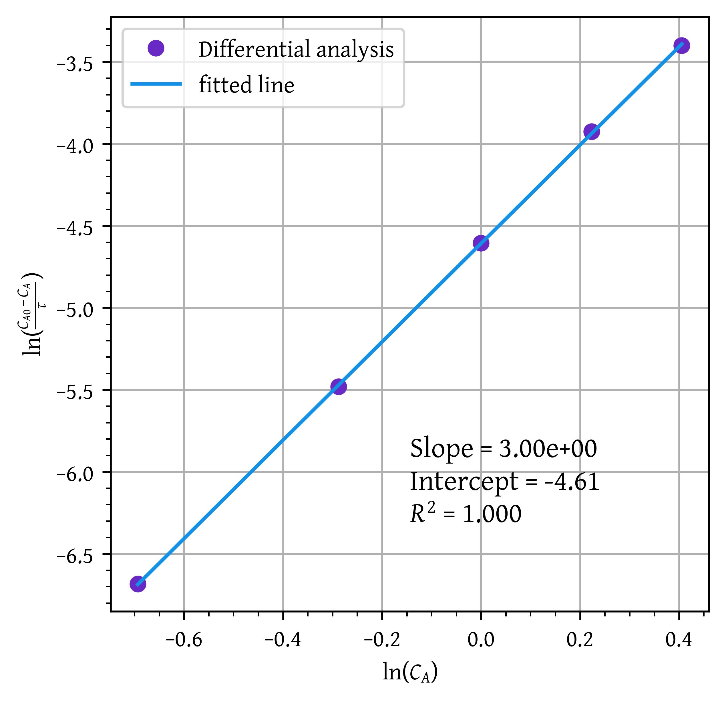
\ce{A -> B + C} is carried out in a CSTR. To learn the rate law, the volumetric flow rate, v_0 , (hence \tau = V / v_0 ) is varied and the effluent concentrations of species A are recorded as a function of the space time t. Pure A enters the reactor at a concentration of 2 mol/ dm³. Steady-state conditions exist when the measurements are recorded.

Run	1	2	3	4	5
\tau (min)	15	38	100	300	1200
CA (mol/dm3)	1.5	1.25	1.0	0.75	0.5

1. Determine the reaction order and specific reaction-rate constant.

2. If you were to repeat this experiment to determine the kinetics, what would you do differently? Would you run at a higher, lower, or the same temperature? If you were to take more data, where would you place the measurements (e.g., \tau )?

3. It is believed that the technician may have made a dilution factor-of-10 error in one of the concentration measurements. What do you think? How do your answers compare using regression (Polymath or other software) with those obtained by graphical methods?

Note: All measurements were taken at steady-state conditions.

Solution

• The liquid-phase irreversible reaction

\ce{A -> B + C}

• carried out in a CSTR.

• \tau vs. C_A data is given

Rate law: -r_A = k C_A^\alpha

For CSTR,

V = \frac{\upsilon_0 (C_{A0} - C_A)}{-r_A} \Rightarrow \tau = \frac{(C_{A0} - C_A)}{k C_A^\alpha}

\therefore k C_A^\alpha = \frac{(C_{A0} - C_A)}{\tau}

Taking log \ln k + \alpha \ln C_A = \ln \left(\frac{C_{A0} - C_A}{\tau} \right)

import numpy as np
from scipy.stats import linregress
import matplotlib.pyplot as plt

# Data
C_A0 = 2.0  # mol/dm^3

tau = np.array([15, 38, 100, 300, 1200])  # space time in minutes
C_A = np.array([1.5, 1.25, 1.0, 0.75, 0.5])  # concentration in mol/dm^3

# plot the data
plt.plot(tau, C_A, 'o-', label='concentration')
plt.xlabel('$\\tau$')
plt.ylabel('$C_A$')

plt.legend()
plt.grid(True)
plt.xlim(0,1200)

plt.show()


ln_ca = np.log(C_A)
ln_ca_by_tau = np.log((C_A0 - C_A)/ tau)

# fit line
res = linregress(ln_ca, ln_ca_by_tau)
line = res.slope * ln_ca + res.intercept

plt.plot(ln_ca, ln_ca_by_tau, 'o', label='Differential analysis')
plt.plot(ln_ca, line, '-', label='fitted line')

plt.annotate(
  f'Slope = {res.slope:.2e}\nIntercept = {res.intercept:.2f}\n$R^2$ = {res.rvalue**2:.3f}',
  xy=(0.5, 0.15),
  xycoords='axes fraction',
  fontsize=12
)

plt.xlabel('$\ln (C_A)$')
plt.ylabel('$\ln(\\frac{C_{A0}-C_A}{\\tau})$')

plt.legend()
plt.grid(True)

plt.show()

# pick the closest round order
order = round(res.slope)
k = np.exp(res.intercept)

Reaction order is = 3, and k is 9.971e-03 1/s.

P 7-6

The reaction

\ce{ A -> B + C }

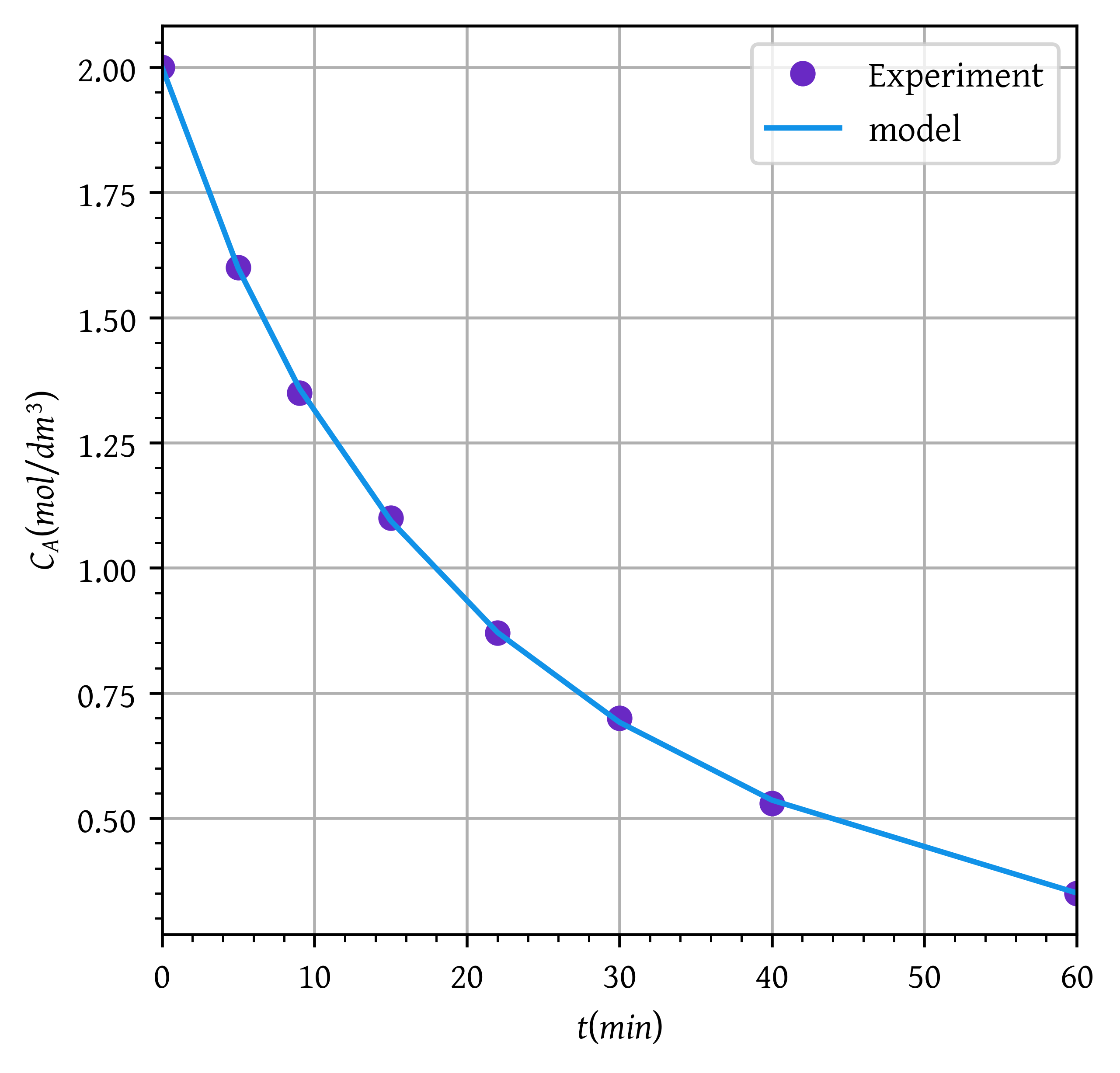
was carried out in a constant-volume batch reactor where the following concentration measurements were recorded as a function of time.

t (min)	0	5	9	15	22	30	40	60
CA (mol/dm3)	2	1.6	1.35	1.1	0.87	0.70	0.53	0.35

1. Use nonlinear least squares (i.e., regression) and one other method to determine the reaction order, \alpha, and the specific reaction rate, k.

2. Nicolas Bellini wants to know, if you were to take more data, where would you place the points? Why?

3. Prof. Dr. Sven Köttlov from Jofostan University always asks his students, if you were to repeat this experiment to determine the kinetics, what would you do differently? Would you run at a higher, lower, or the same temperature? Take different data points? Explain.

4. It is believed that the technician made a dilution error in the concentration measured at 60 min.

What do you think? How do your answers compare using regression (Polymath or other software) with those obtained by graphical methods?

Solution

Reaction: \ce{ A -> B + C }

• carried out in a constant-volume batch reactor

-\frac{dC_A}{dt} = k C_A^\alpha

• concentration measurements were recorded as a function of time.

import numpy as np
from scipy.integrate import solve_ivp
from scipy.optimize import minimize

from scipy.optimize import curve_fit
import matplotlib.pyplot as plt

# Given data
t = np.array([0, 5, 9, 15, 22, 30, 40, 60])  # min
C_A = np.array([2, 1.6, 1.35, 1.1, 0.87, 0.7, 0.53, 0.35])  # mol/dm^3

C_A0 = C_A[0]

# Define the system of ODEs
def batch_reactor(t, y, *args):
    C_A = y[0]
    k, n = args
    
    rate = -k*C_A**n
    dca_dt = rate

    return [dca_dt]


t_span = (t.min(), t.max())

# initial conditions
y0 = [C_A0]

# Initial guesses of k and n
k = 1 
n = 1

# Objective function to minimize: the difference between C_A (experimental) and C_A (model)

def objective(params):
    k,n = params

    # Solve the ODE using solve_ivp
    solution = solve_ivp(
      batch_reactor,        # The ODE function to solve
      t_span,              # Time interval
      y0,               # Initial condition in a list
      args=(k, n),         # Additional arguments passed to the ODE function
      dense_output=True    # Generate a continuous solution
    )

    sol_specific = solution.sol(t)
    C_A_model = solution.sol(t)[0] 

    ssr = np.sum((C_A - C_A_model)**2)  # Sum of squared residuals

    return ssr

# Minimize the objective function
result = minimize(objective, [k,n], bounds=[(1e-4, 1e4), (0, 5)])

# Extract the results
k_opt, n_opt = result.x
success = result.success

# Check if the solution was successful
if not success:
    print("Optimization was not successful. Try different initial guesses or methods.")

final_solution = solve_ivp(
  batch_reactor,        # The ODE function to solve
  t_span,              # Time interval
  y0,               # Initial condition in a list
  args=(k_opt, n_opt),         # Additional arguments passed to the ODE function
  dense_output=True    # Generate a continuous solution
)

C_A_model = final_solution.sol(t)[0] 

# plot the data
plt.plot(t, C_A, 'o', label='Experiment')
plt.plot(t, C_A_model, '-', label='model')
plt.xlabel('$t (min)$')
plt.ylabel('$C_A (mol/dm^3)$')

plt.legend()
plt.grid(True)
plt.xlim(0,60)

plt.show()

Initial guess for Reaction order is = 1.00, and k is 1.000e+00.

Optimized value of Reaction order is = 1.52, and k is 3.305e-02.

P 7-7

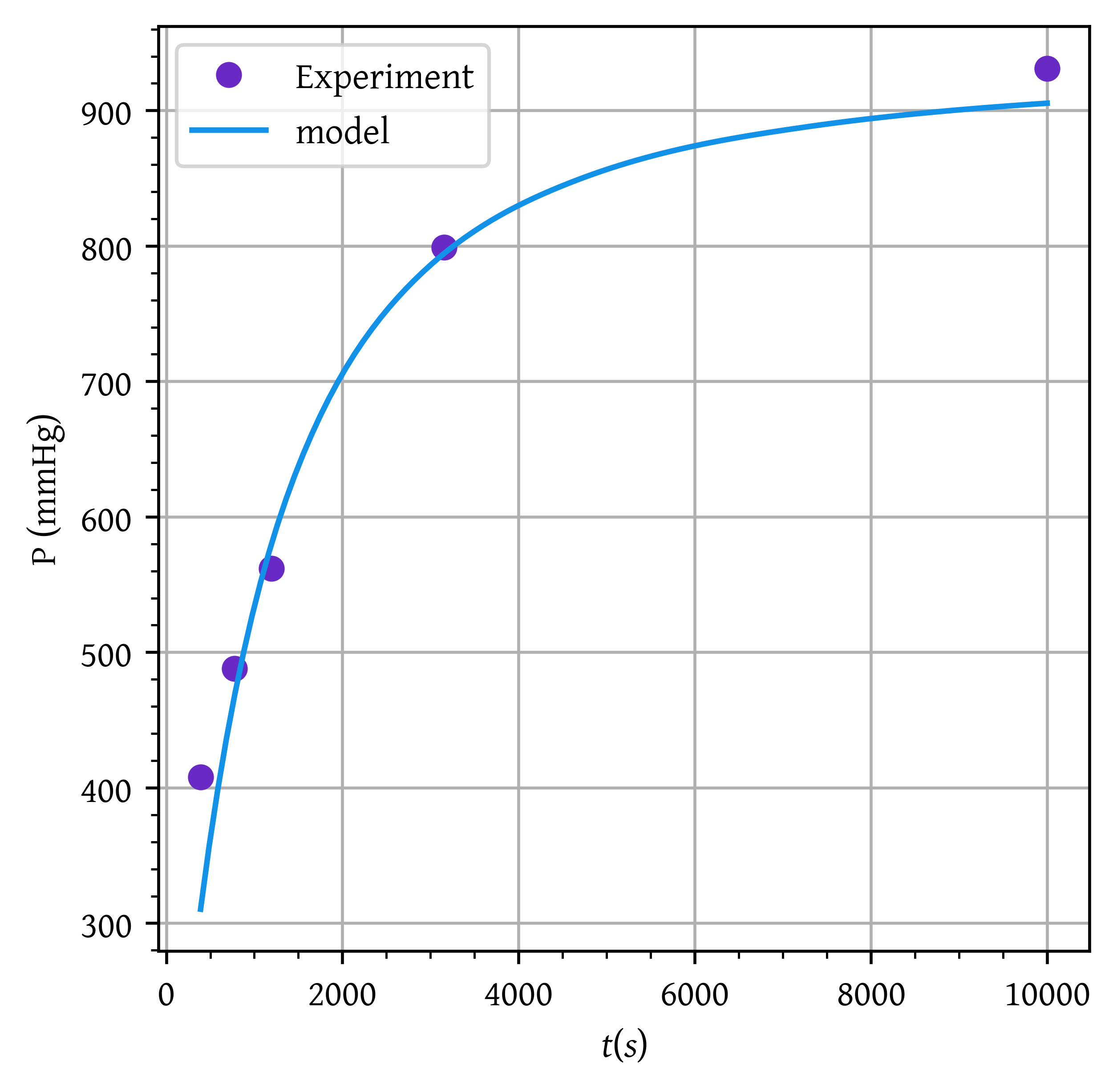
The following data were reported [from C. N. Hinshelwood and P. J. Ackey, Proc. R. Soc. (Lond)., A115, 215] for a gas-phase constant-volume decomposition of dimethyl ether at 504^{\circ}C in a batch reactor. Initially, only \ce{(CH3)2O} was present.

Time (s)	390	777	1195	3155	\infty
Total Pressure (mmHg)	408	488	562	799	931

1. Why do you think the total pressure measurement at t = 0 is missing? Can you estimate it?

2. Assuming that the reaction

\ce{(CH3)2O -> CH4 + H2 + CO}

is irreversible and goes virtually to completion, determine the reaction order and specific reaction rate k.

3. What experimental conditions would you suggest if you were to obtain more data?

4. How would the data and your answers change if the reaction were run at a higher temperature? A lower temperature?

Solution

• constant volume batch reactor

• Data on pressure with time is given

\ce{(CH3)2O -> CH4 + H2 + CO}

y_{A0} = 1

\delta = 3 - 1 = 2

\epsilon = y_{A0} \delta = 2

V = V_0 = V_0 \frac{P_0}{P} (1 + \epsilon X)

P = P_0 (1 + \epsilon X)

X = \frac{P - P_0}{\epsilon P_0}

At t = \infty, X = 1

P_\infty = P_0 (1 + 2) 3 P_0

P_0 = P_\infty/3

Rate law: -r_A = k C_A^\alpha

As pressure data is given, we need an equation for dP/dt

dP/dt = d/dt (P_0 (1 + \epsilon X))

dP/dt = P_0 \epsilon dX/dt

• For constant volume batch reactor

\frac{dC_A}{dt} = -k C_A^\alpha

C_A = C_{A0}^\alpha (1-X)^\alpha

\frac{dX}{dt} = k (1-X)^\alpha

import numpy as np
from scipy.integrate import solve_ivp
from scipy.optimize import minimize

from scipy.optimize import curve_fit
import matplotlib.pyplot as plt

# Given data

delta = 2
y_A0 = 1
epsilon = y_A0 * delta

t = np.array([390, 777, 1195, 3155, 10000])  # s, Replace infinity with a large number
P = np.array([408, 488, 562, 799, 931]) # mmHg

P0 = P[-1]/(1 + epsilon)

t_eval = t[:-1]
P_eval = P[:-1]

# Define the system of ODEs
def batch_reactor(t, y, *args):
    p = y[0]
    k, n = args
   
    X = (p-P0)/(epsilon * P0)

    dxdt = k * (1-X)**n
    dpdt = P0 * epsilon* dxdt

    return [dpdt]

t_span = (min(t_eval), max(t_eval))

# initial conditions
y0 = [P0]

# Initial guesses of k and n
k = 6e-4
n = 1

# Objective function to minimize: the difference between C_A (experimental) and C_A (model)

def objective(params):
    k,n = params

    # Solve the ODE using solve_ivp
    solution = solve_ivp(
      batch_reactor,        # The ODE function to solve
      t_span,              # Time interval
      y0,               # Initial condition in a list
      args=(k, n),         # Additional arguments passed to the ODE function
      dense_output=True    # Generate a continuous solution
    )

    P_model = solution.sol(t_eval)[0] 

    ssr = np.sum((P_eval - P_model)**2)  # Sum of squared residuals

    return ssr

# Minimize the objective function
result = minimize(objective, [k,n], bounds=[(1e-4, 1e-3), (0, 2)])

# Extract the results
k_opt, n_opt = result.x
success = result.success

# Check if the solution was successful
if not success:
    print("Optimization was not successful. Try different initial guesses or methods.")

t_span = (min(t), max(t))

final_solution = solve_ivp(
  batch_reactor,        # The ODE function to solve
  t_span,              # Time interval
  y0,               # Initial condition in a list
  args=(k_opt, n_opt),         # Additional arguments passed to the ODE function
  dense_output=True    # Generate a continuous solution
)

t_plot = np.linspace(t.min(), t.max(),100) 
P_model = final_solution.sol(t_plot)[0] 

# plot the data
plt.plot(t, P, 'o', label='Experiment')
plt.plot(t_plot, P_model, '-', label='model')
plt.xlabel('$t (s)$')
plt.ylabel('P (mmHg)')

plt.legend()
plt.grid(True)

plt.show()

Initial guess for Reaction order is = 1.00, and k is 6.000e-04.

Optimized value of Reaction order is = 1.50, and k is 8.184e-04.

P 7-10

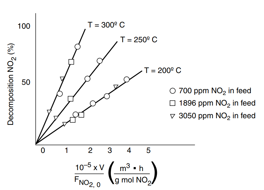
Tests were run on a small experimental reactor used for decomposing nitrogen oxides in an automobile exhaust stream. In one series of tests, a nitrogen stream containing various concentrations of \ce{NO2} was fed to a reactor, and the kinetic data obtained are shown in Figure P7-10. Each point represents one complete run. The reactor operates essentially as an isothermal backmix reactor (CSTR). What can you deduce about the apparent order of the reaction over the temperature range studied?

Figure 1: Figure P7-10 - Auto exhaust data.

The plot gives the fractional decomposition of \ce{NO2} fed versus the ratio of reactor volume V (in cm³) to the NO₂ feed rate, F_{NO_{2,0}} (g mol/h), at different feed concentrations of \ce{NO2} (in parts per million by weight). Determine as many rate law parameters as you can.

Solution

X = \frac{\text{\% decomposition}}{100}

Rate law: -r_A = kC_A^n

• V/F_{A0} vs. X data is given

• Reaction carried out in CSTR

V = \frac{F_{A0}X}{-r_A}

\frac{V}{F_{A0}} = \frac{X}{k C_A^n}

The linear nature of experiment at a given temperature in Figure 1 indicates that X \propto \frac{V}{F_{A0}}

Therefore, apparent order must be zero (C_A^n = 1).

k \frac{V}{F_{A0}} = X

References

Fogler, H. Scott. 2016. Elements of Chemical Reaction Engineering. Fifth edition. Boston: Prentice Hall.