Workshop 02 Solution: Conversion and reactor sizing
Lecture notes for chemical reaction engineering
Problem 1
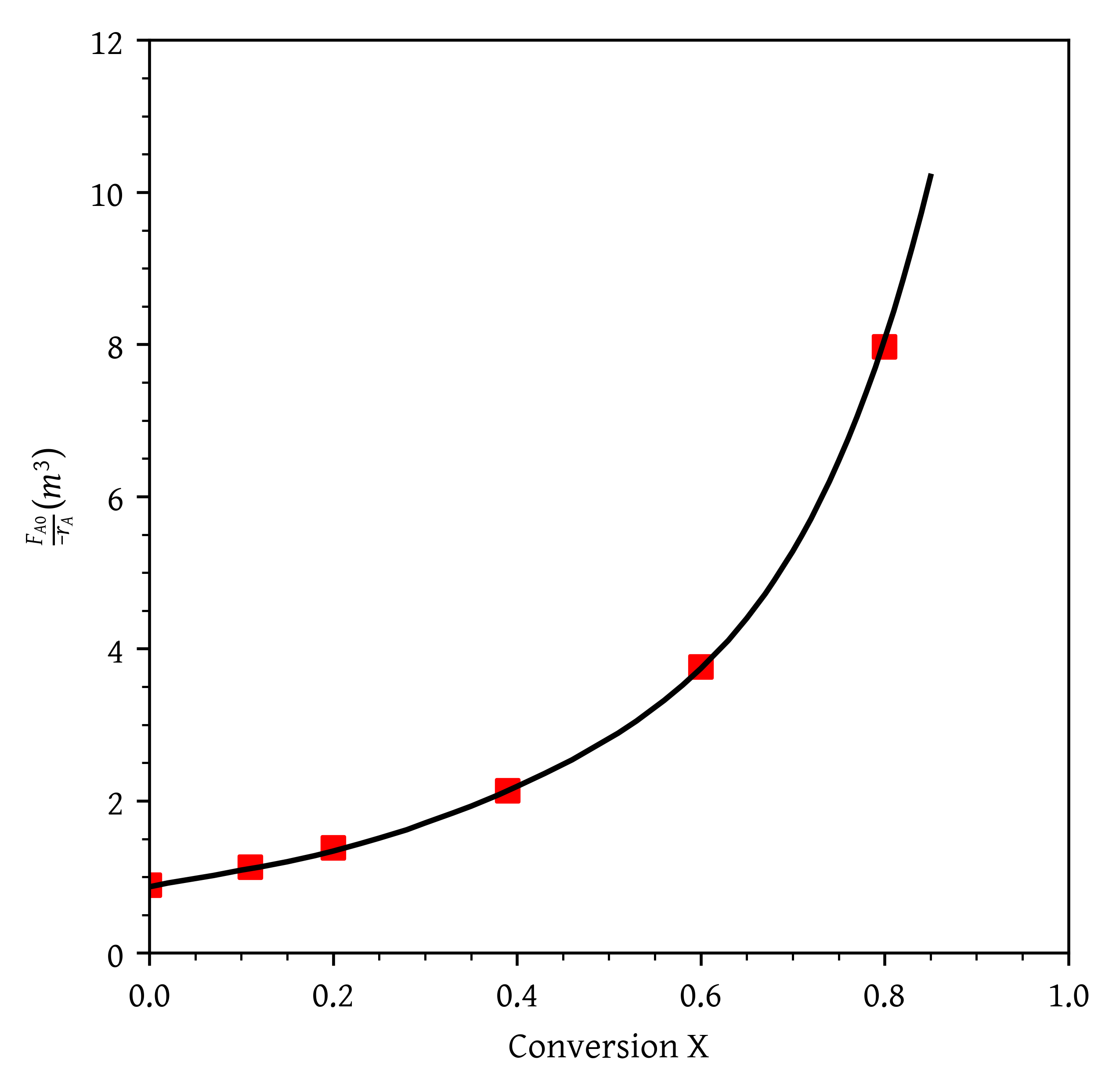
P2-3: You have two CSTRs and two PFRs, each with a volume of 1.6 m^3 . Use Figure 1 to calculate the conversion for each of the reactors in the following arrangements.
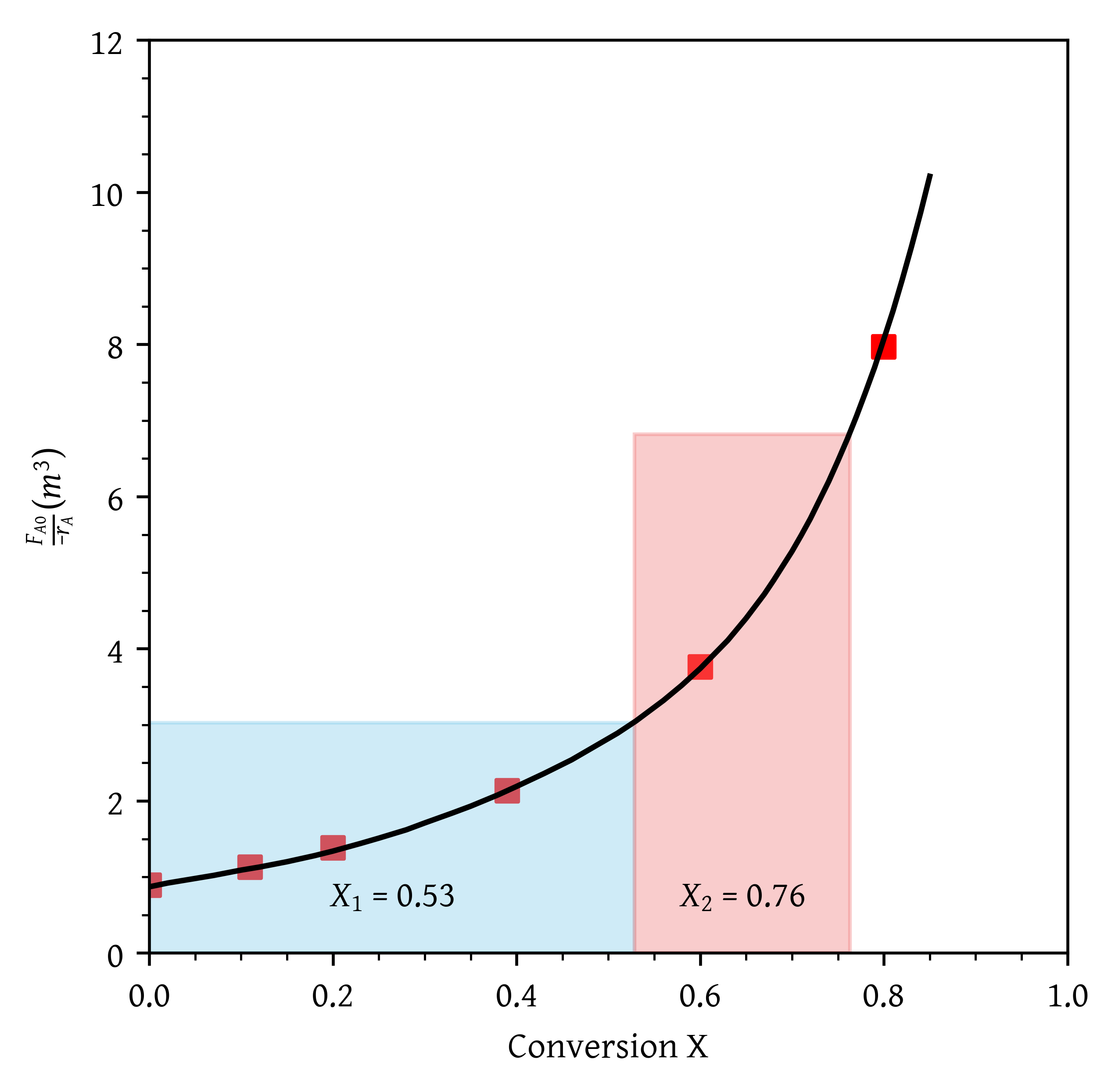
- Two CSTRs in series.
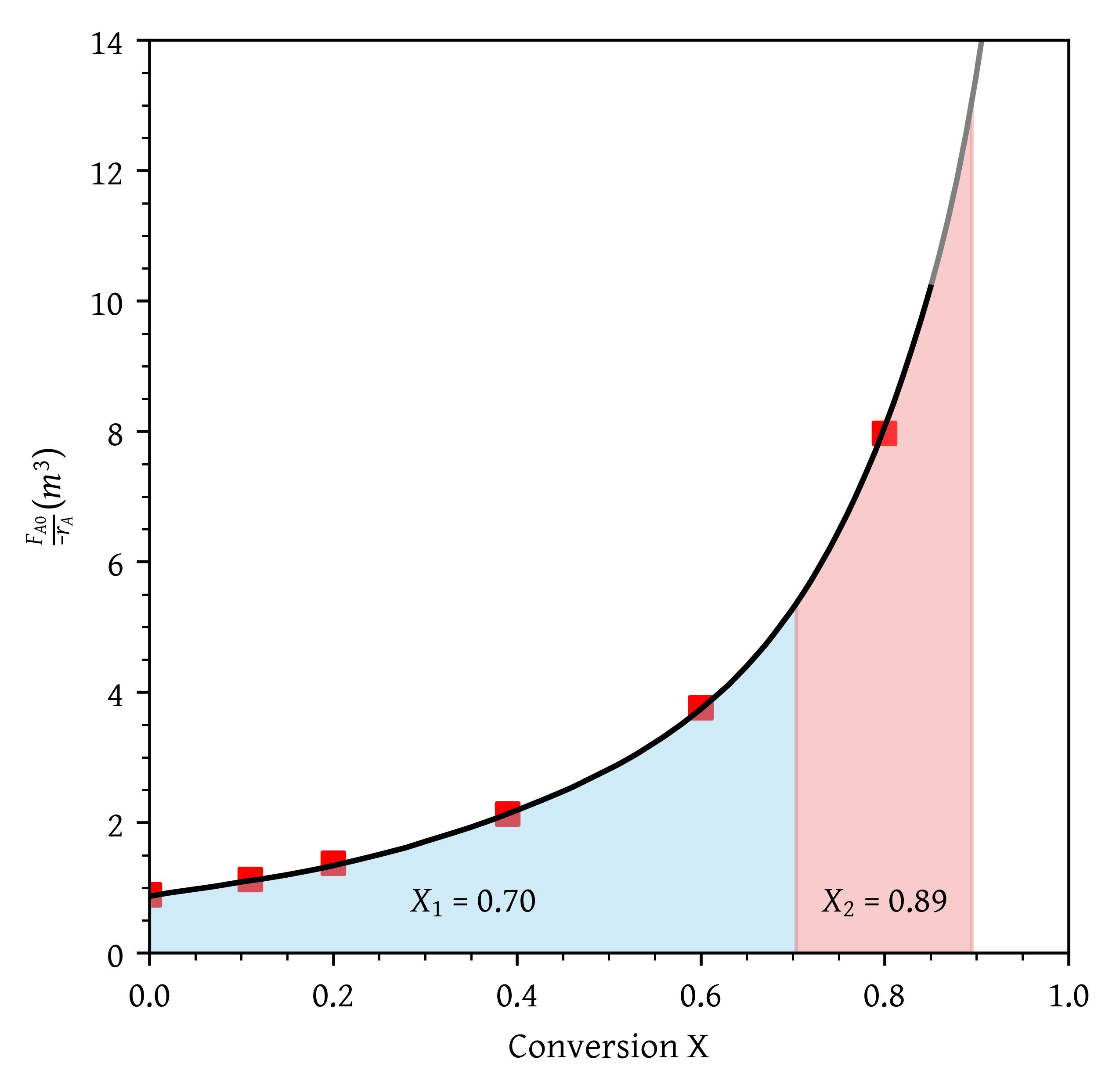
- Two PFRs in series.
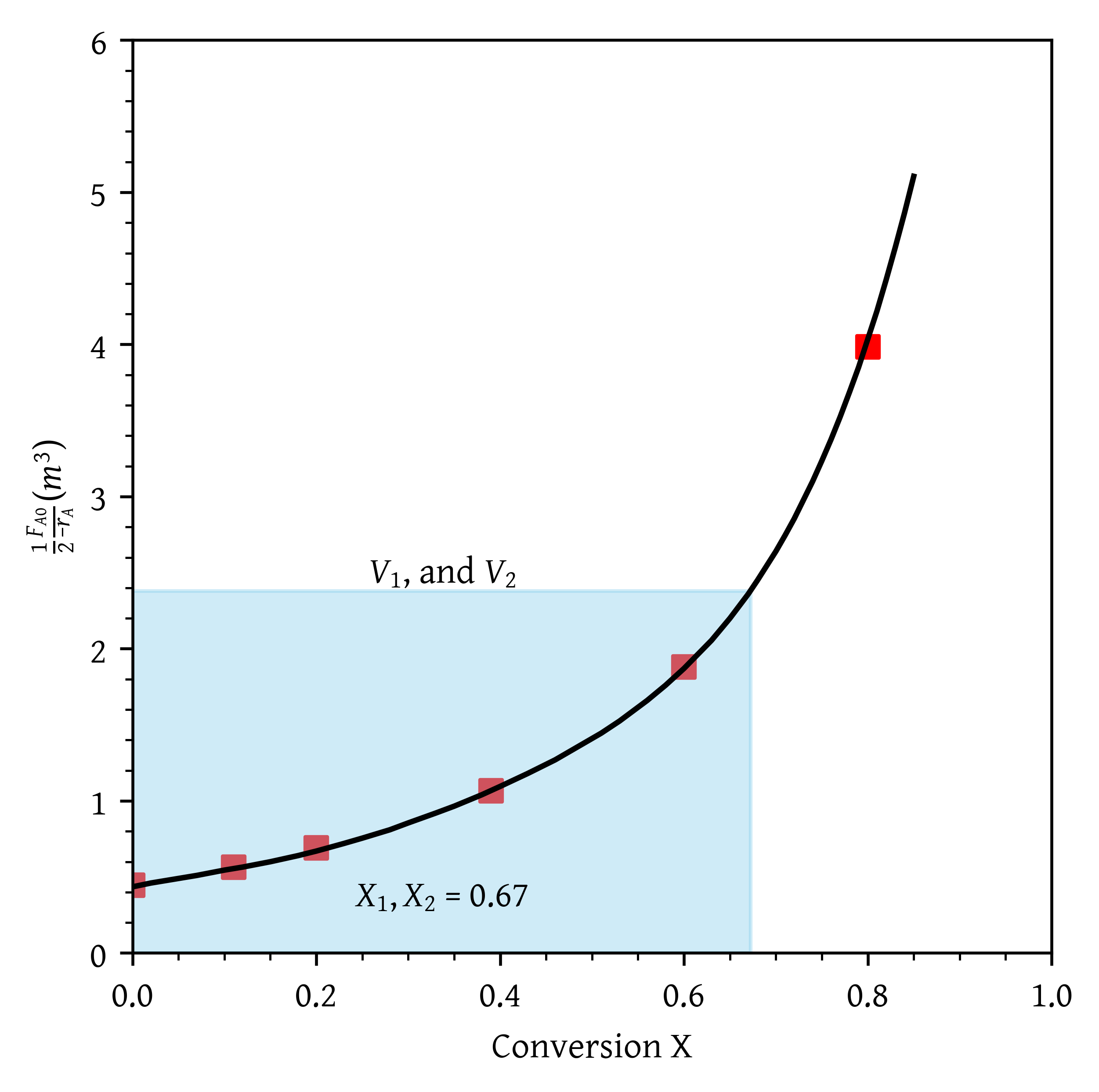
- Two CSTRs in parallel with the feed, F_{A0}, divided equally between the two reactors.
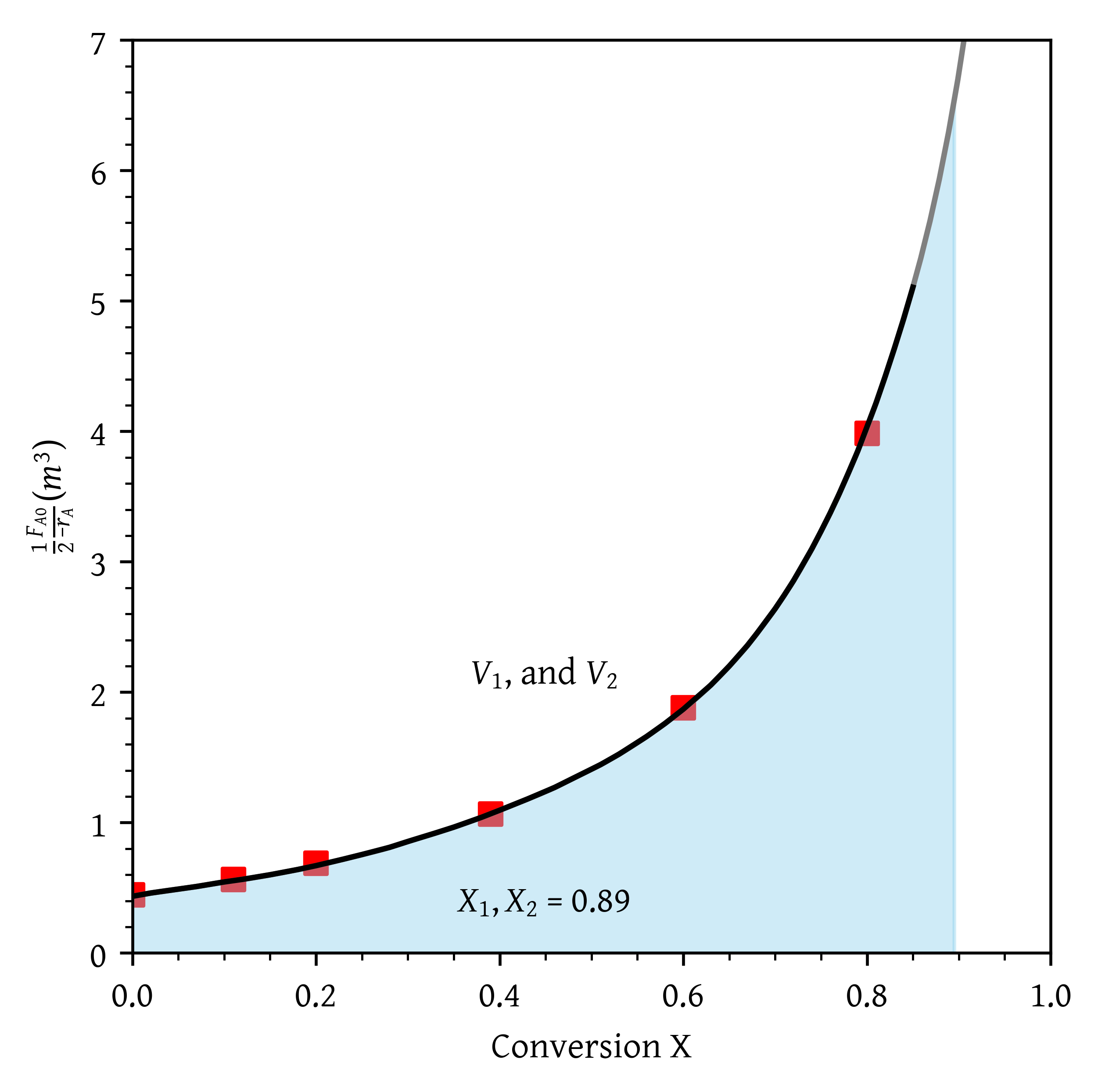
- Two PFRs in parallel with the feed divided equally between the two reactors.
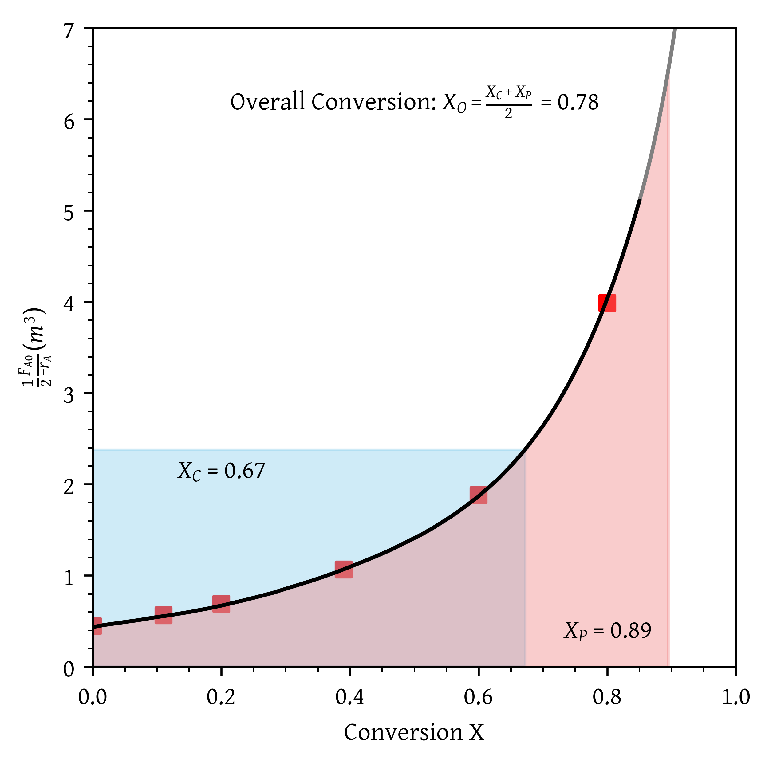
- A CSTR and a PFR in parallel with the flow equally divided. Calculate the overall conversion, X_{ov}
X_{ov} = \frac{F_{A0}-F_{A,CSTR} - F_{A,PFR}}{F_{A0}} with F_{A,CSTR} = \frac{F_{A0}}{2} - \frac{F_{A0}}{2} X_{CSTR} , \text{and } F_{A,PFR} = \frac{F_{A0}}{2} (1 - X_{PFR})
- A PFR followed by a CSTR.
- A CSTR followed by a PFR.
- A PFR followed by two CSTRs. Is this arrangement a good arrangement or is there a better one?
Solution:
To read the CSV file use the genfromtxt function from numpy
import numpy as np

p1_expt_file = './workshop-02-problem-1-data.csv'
p1_expt_data = np.genfromtxt(p1_expt_file,
                             delimiter=',',
                             dtype=[('x', float),
                                    ('fa0_by_ra', float)],
                             skip_header=1)
To interpolate the data, use CubicSpline function from scipy.interpolate.
import scipy.interpolate as interpolate

p1_interp = interpolate.CubicSpline(p1_expt_data['x'],
                                    p1_expt_data_data['fa0_by_ra'])
Data plotting using matplotlib.pyplot
import matplotlib.pyplot as plt

fig,ax = plt.subplots()

ax.scatter(p1_expt_data['x'],
           p1_expt_data['fa0_by_ra'],
           marker='s',
           color='red')

ax.set_xlabel('Conversion X')
ax.set_ylabel('$\\frac{F_{A0}}{-r_A} (m^3)$')

# Setting x and y axis limits
ax.set_xlim(0, 1)
ax.set_ylim(0, 12)

plt.show()
Add fit line to the plot
x_interp =np.linspace(0,1,100)
ax.plot(x_interp, p1_interp(x_interp), color='grey')
Add rectangle to the plot
# Adds rectangle from (0,0) with a width of x1 and height of y1
rectangle = plt.Rectangle((0, 0), x1, y1, color='skyblue', alpha=0.4)
ax.add_patch(rectangle)
Color area under the curve
 Fill the area under the curve between x1 and x2
x_fill = np.linspace(x1, x2, 100)
y_fill = p1_interp(x_fill)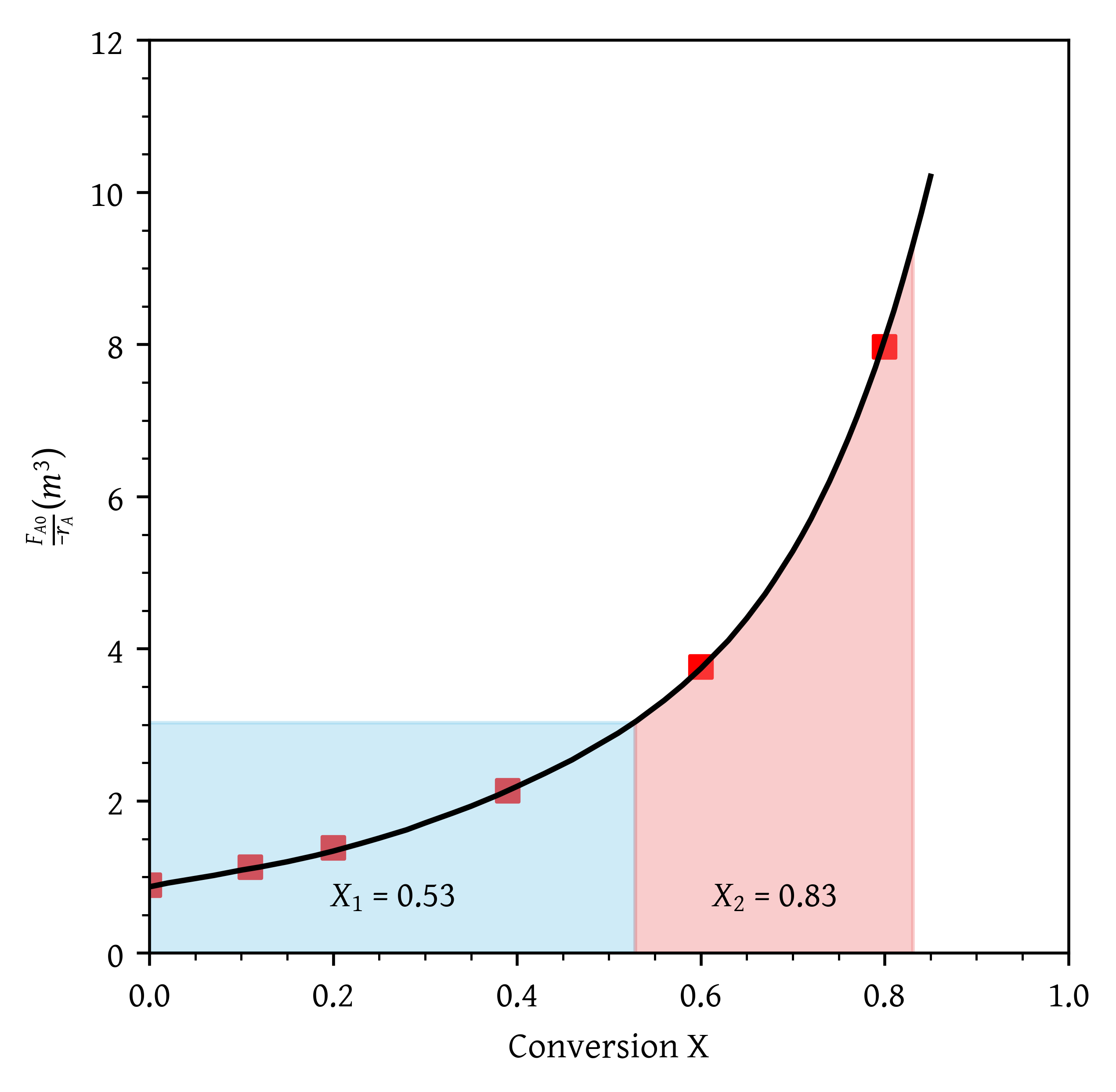
ax.fill_between(x_fill, y_fill, color='skyblue', alpha=0.4)- Two CSTRs in series (Figure 3).
- Two PFRs in series (Figure 4).
- Two CSTRs in parallel with the feed, F_{A0}, divided equally between the two reactors (Figure 5).
- Two PFRs in parallel with the feed divided equally between the two reactors (Figure 6).
- A CSTR and a PFR in parallel with the flow equally divided. Calculate the overall conversion, X_{ov} (Figure 7)
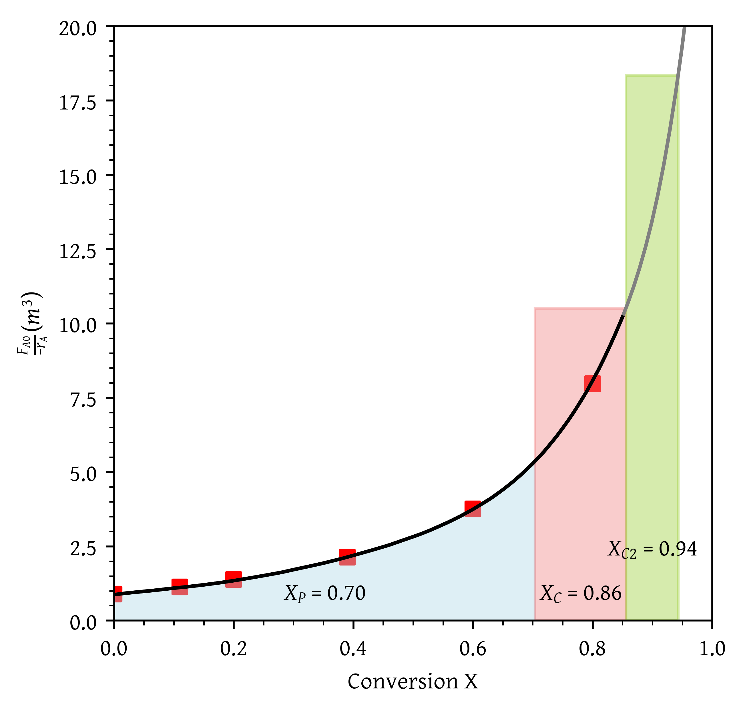
- A PFR followed by a CSTR (Figure 8).
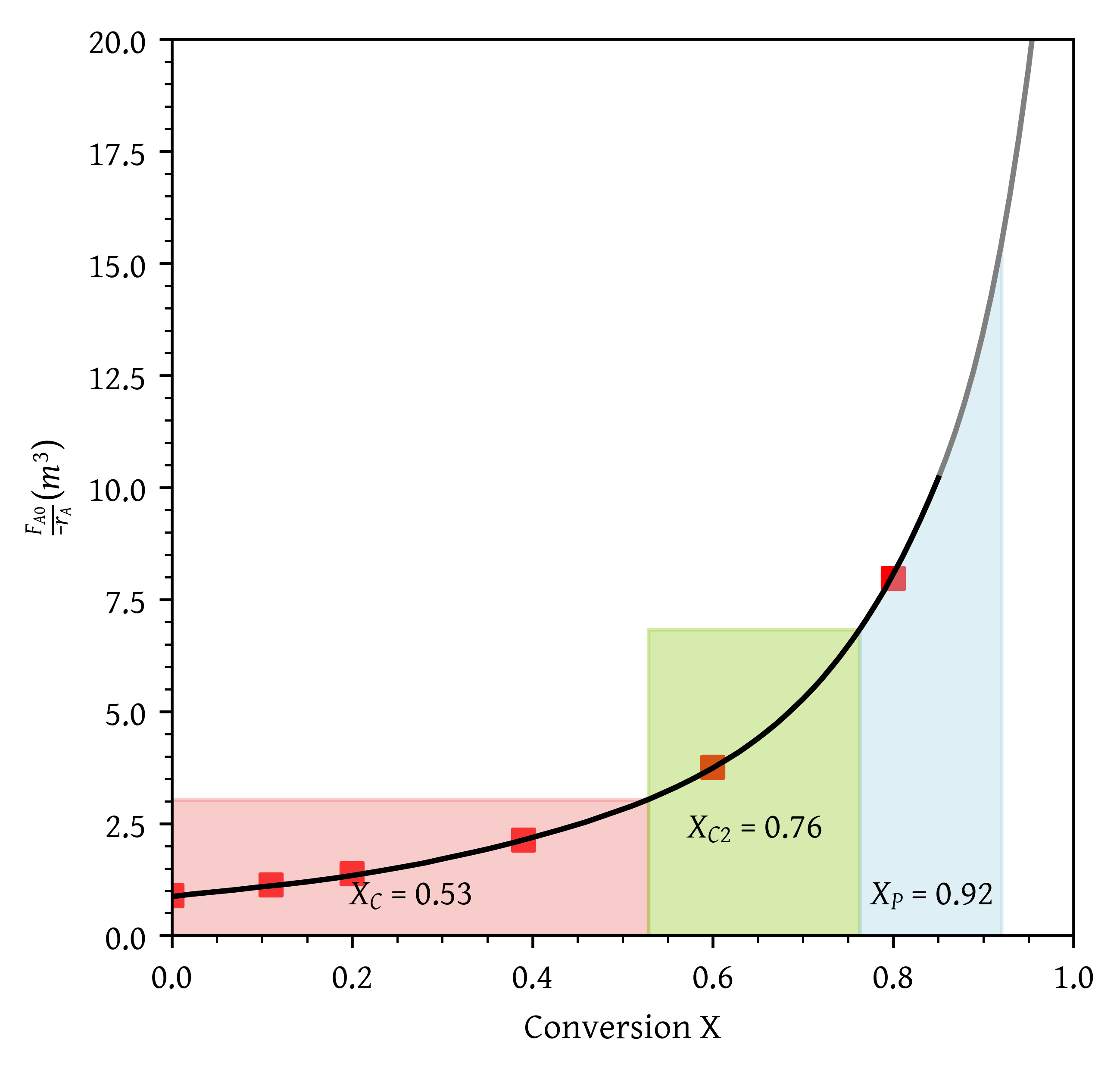
- A CSTR followed by a PFR (Figure 9).
- A PFR followed by two CSTRs (Figure 10). Is this arrangement a good arrangement or is there a better one?
Two CSTRs followed by a PFR (Figure 11) yield final conversion of X_3 = 0.92.
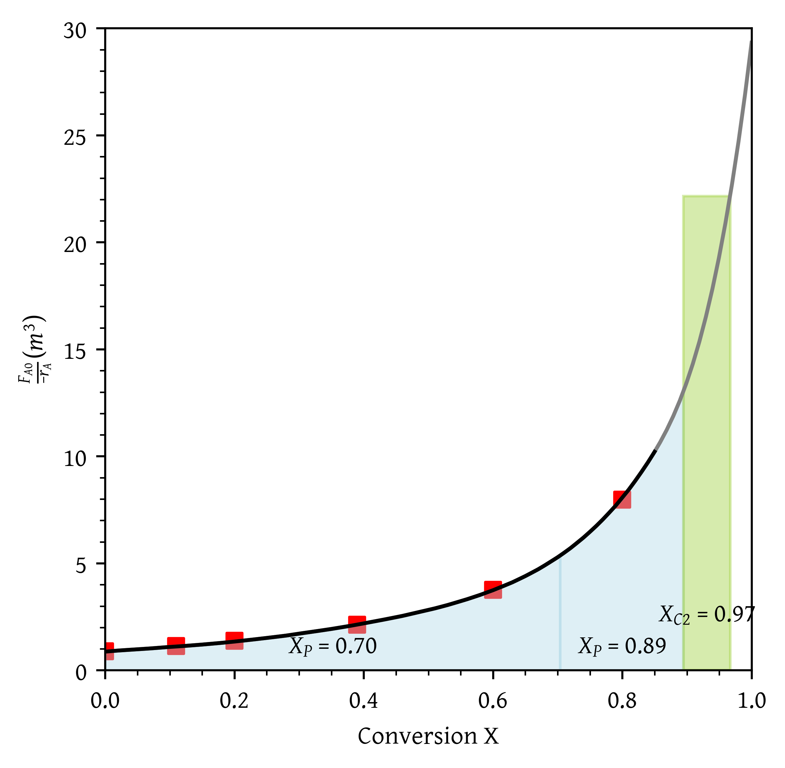
Two PFRs followed by a CSTR (Figure 12) yield final conversion of X_3 = 0.97.
Problem 2
P2-4: The exothermic reaction of stillbene (A) to form the economically important trospophene (B) and methane (C), i.e.,
\ce{A -> B + C}
was carried out adiabatically and the following data recorded:
| X | -r_A (mol/dm^3 min) |
|---|---|
| 0 | 1 |
| 0.2 | 1.67 |
| 0.4 | 5 |
| 0.45 | 5 |
| 0.5 | 5 |
| 0.6 | 5 |
| 0.8 | 1.25 |
| 0.9 | 0.91 |
The entering molar flow rate of A was 300 mol/min.
- What are the PFR and CSTR volumes necessary to achieve 40% conversion?
- Over what range of conversions would the CSTR and PFR reactor volumes be identical?
- What is the maximum conversion that can be achieved in a 105 dm^3 CSTR?
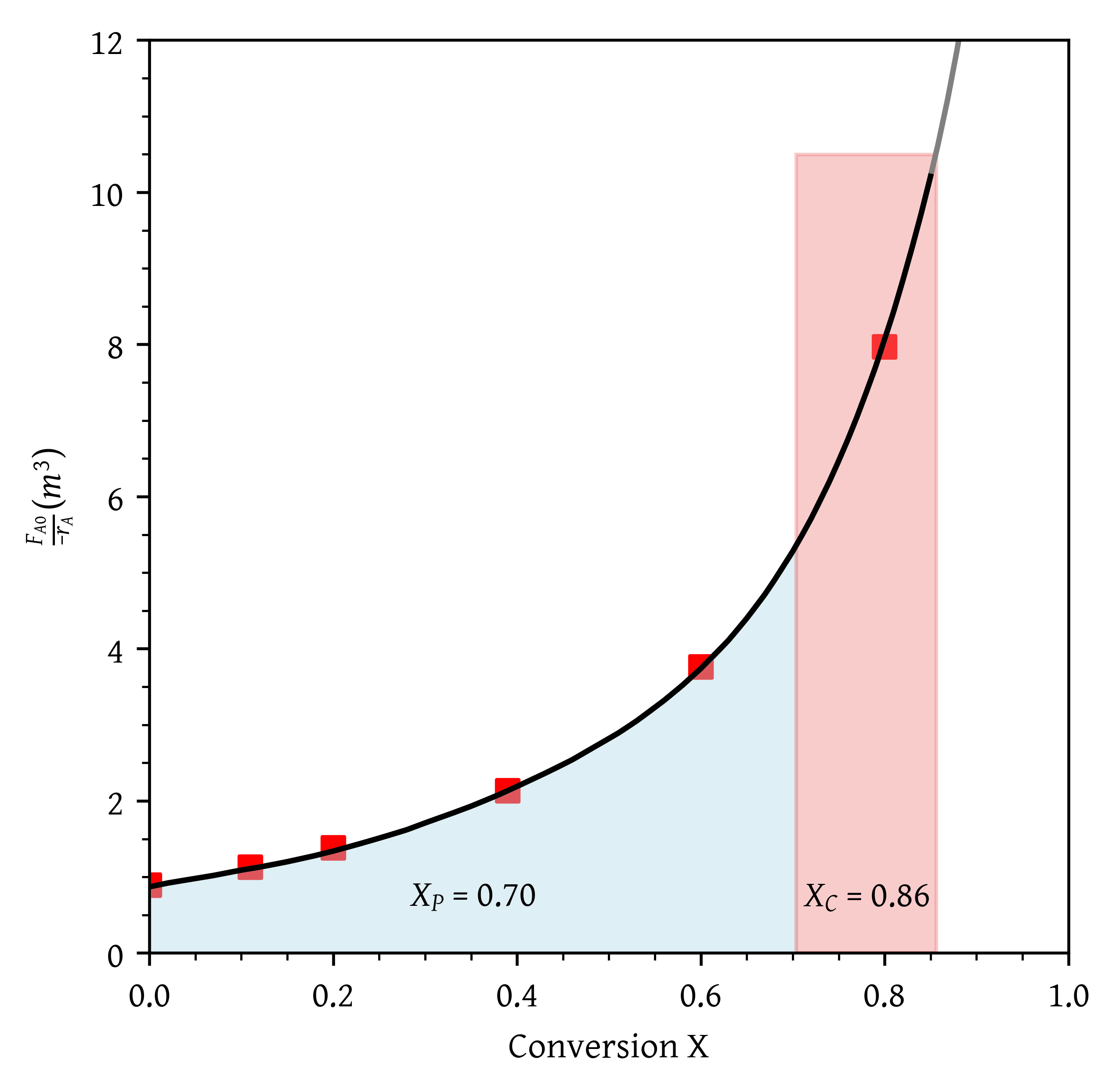
- What conversion can be achieved if a 72 dm^3 PFR is followed in series by a 24 dm^3 CSTR?
- What conversion can be achieved if a 24 dm^3 CSTR is followed in a series by a 72 dm^3 PFR?
- Plot the conversion and rate of reaction as a function of PFR reactor volume up to a volume of 100 dm^3.
Solution:
The rate data (-r_A) is given. We need F_{A0}/-r_A. Dividing F_{A0} = 300 by -r_A we get:
| X | -r_A | F_{A0}/-r_A |
|---|---|---|
| 0 | 1 | 300 |
| 0.2 | 1.67 | 179.641 |
| 0.4 | 5 | 60 |
| 0.45 | 5 | 60 |
| 0.5 | 5 | 60 |
| 0.6 | 5 | 60 |
| 0.8 | 1.25 | 240 |
| 0.9 | 0.91 | 329.67 |
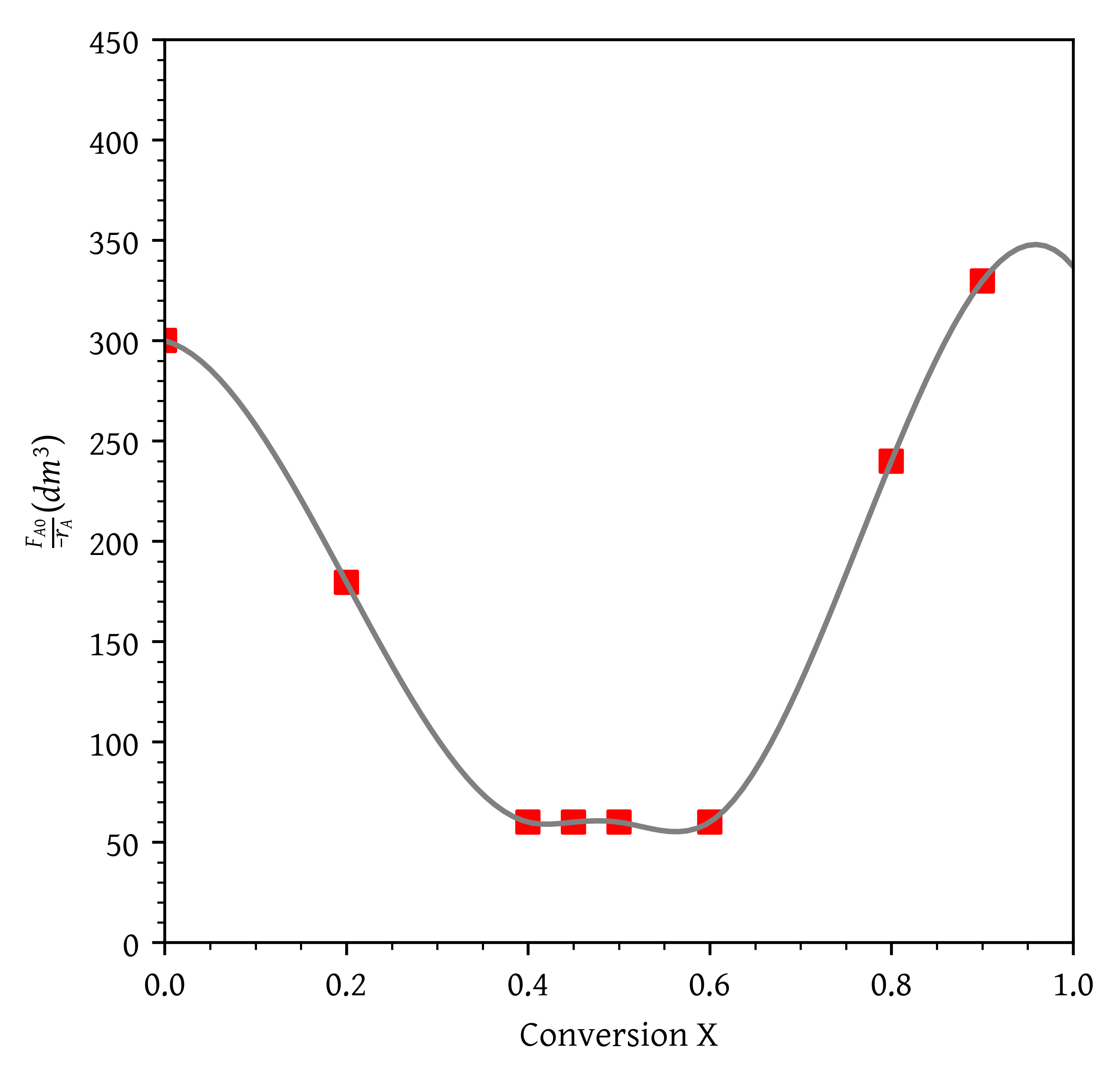
Trying to fit a single cubic spline or a polynomial doesn’t work well due to the nature of the data (Figure 13). The data consists of three liniear segments. Therefore, we fit a piecewise linear function using numpy.piecewise. We also use lambda functions to define the linear segments.
def piecewise_linear_fit(x, x0, y0, k1, k2, k3):
    """
    Piecewise linear function defined by slopes and a constant part.
    x0, y0: Coordinates of the piecewise function's bending points.
    k1, k2, k3: Slopes of the first, second, and third parts.

    Note that in this problem,
    k1 = -600.0
    k2 = 0
    k3 = 898.9010989010986

    x0 = [0.4, 0.6]
    y0 = [60.0, 60.0]

    We can call this function as
    piecewise_linear_fit(x, *args)

    args = ([0.4, 0.6], [60.0, 60.0], -600.0, 0, 898.9010989010986)
    """

    return np.piecewise(x,
                        [x < x0[0], (x >= x0[0]) & (x <= x0[1]), x > x0[1]],
                        [lambda x: k1*x + y0[0] - k1*x0[0],
                         lambda x: y0[1],
                         lambda x: k3*x + y0[1] - k3*x0[1]])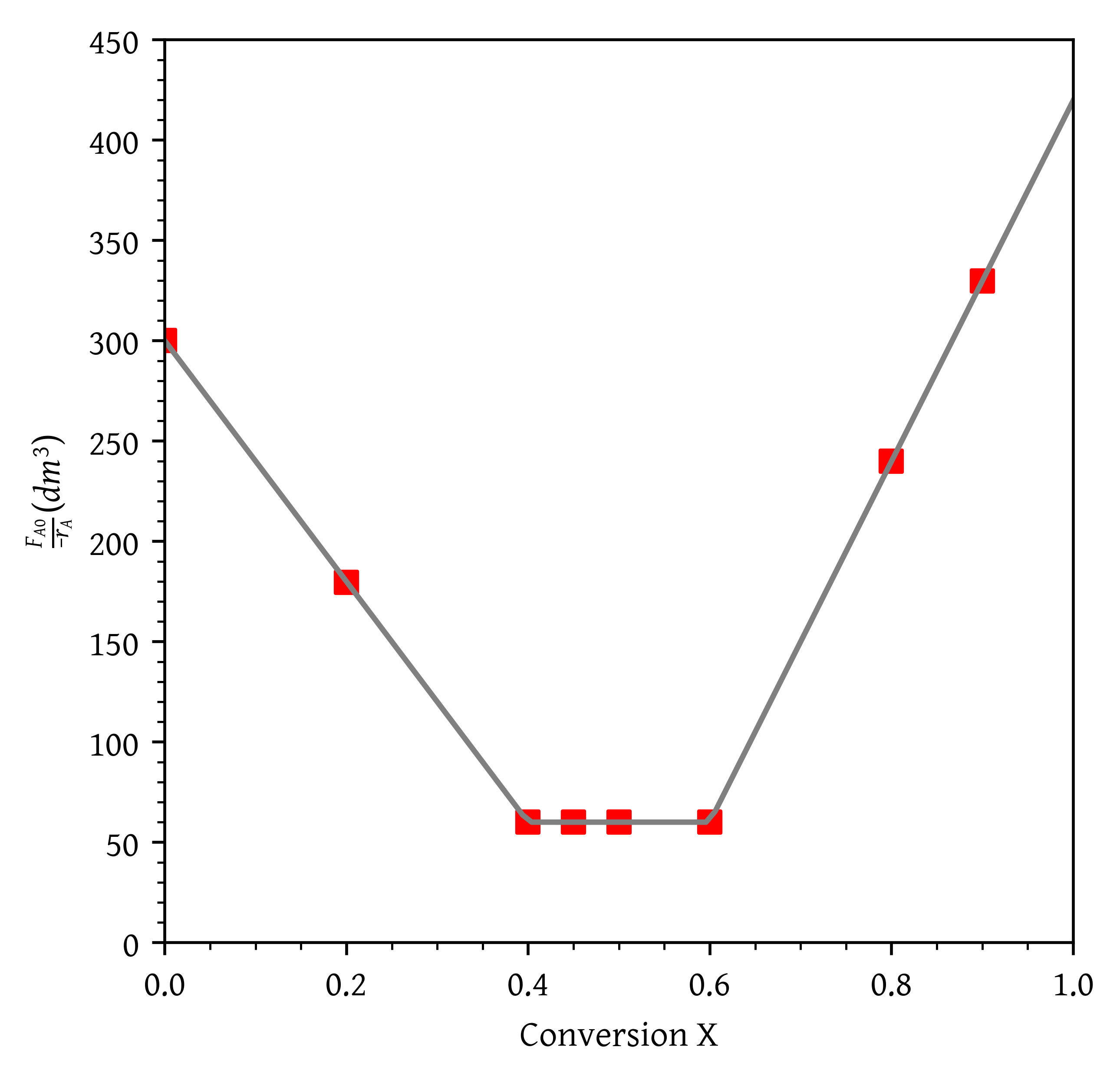
- What are the PFR and CSTR volumes necessary to achieve 40% conversion?
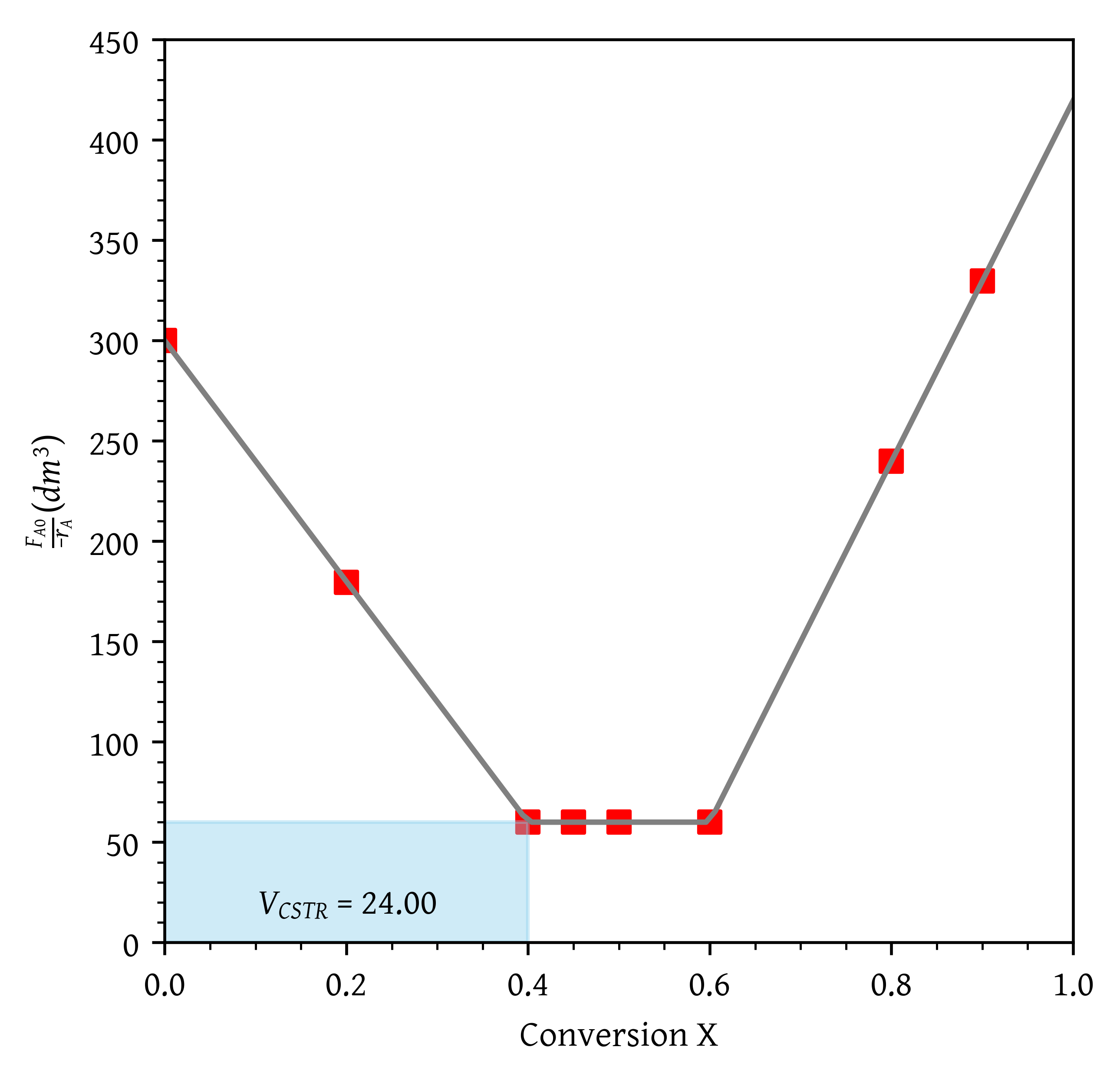
From @fig-problem-2a, $V_{CSTR}$ = 24\.00 $dm^3$.Over what range of conversions would the CSTR and PFR reactor volumes be identical?
As the slope of F_{A0}/-r_A vs.\ X line is 0 between 0.4 and 0.6, the CSTR and PFR volumes over this range would be identical.
What is the maximum conversion that can be achieved in a 105 dm^3 CSTR?
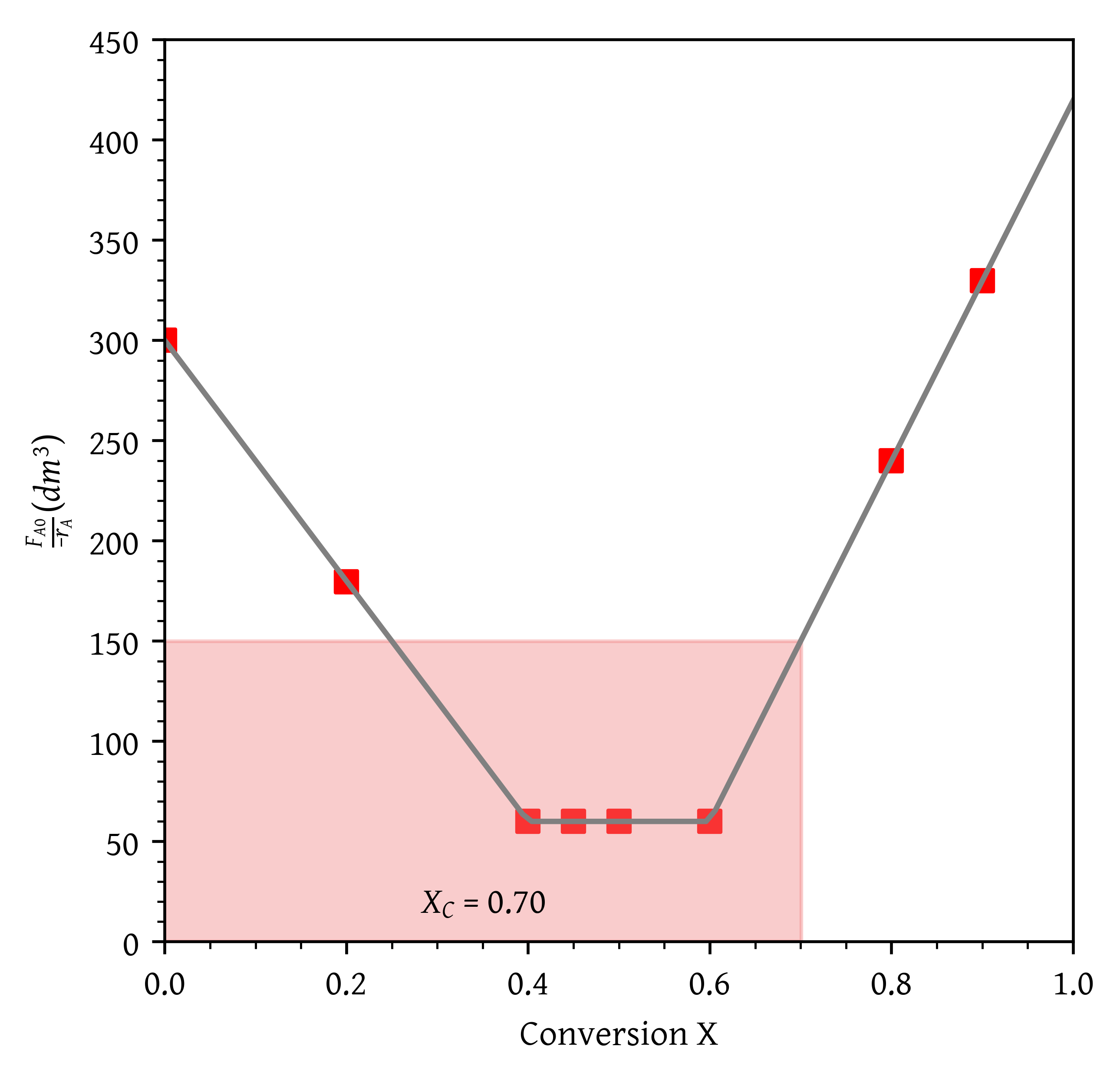
From Figure 16, X = 0.70.
- What conversion can be achieved if a 72 dm^3 PFR is followed in series by a 24 dm^3 CSTR?
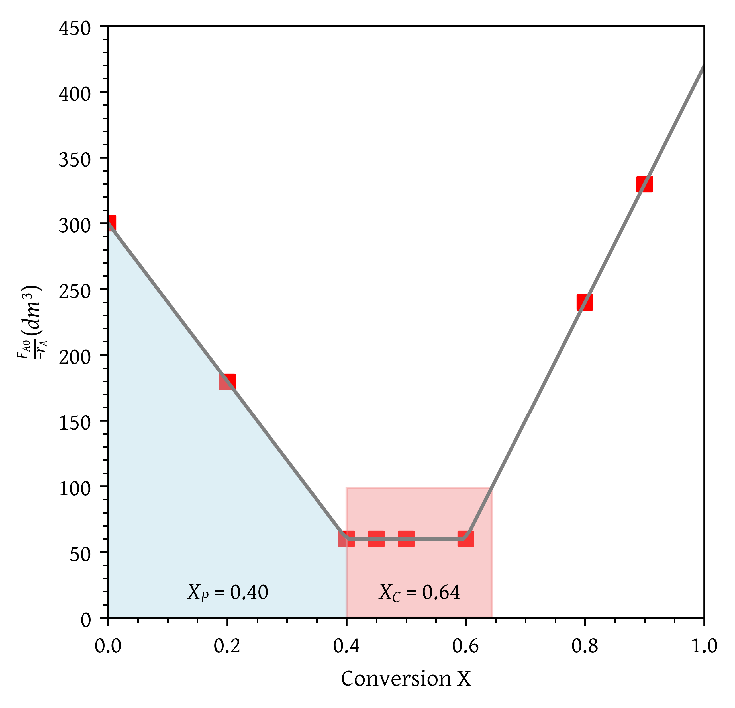
From Figure 17, X_{PFR} = 0.40 and X_{CSTR} = 0.64.
- What conversion can be achieved if a 24 dm^3 CSTR is followed in a series by a 72 dm^3 PFR?
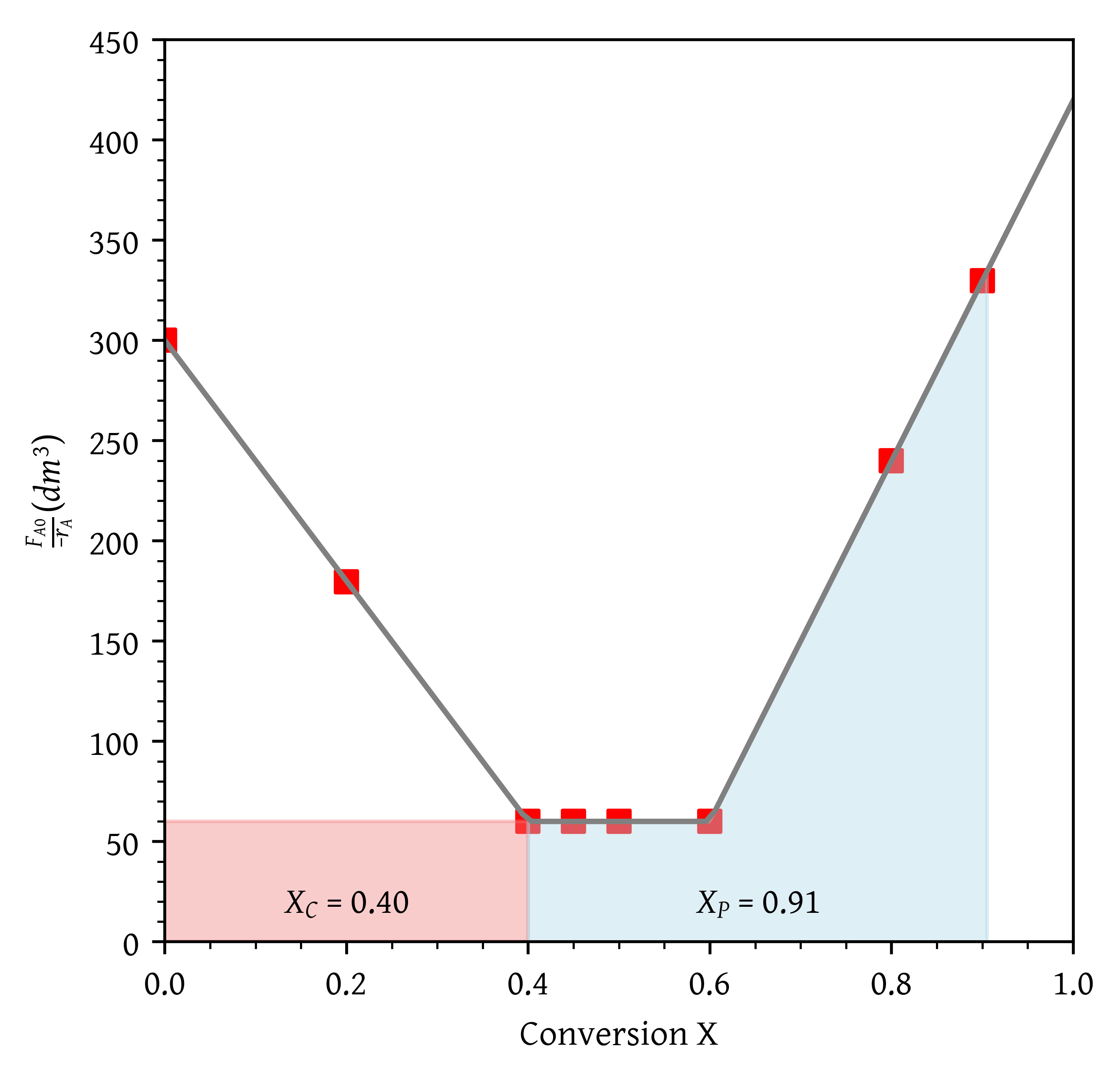
From Figure 18, X_{CSTR} = 0.40 and X_{PFR} = 0.91.
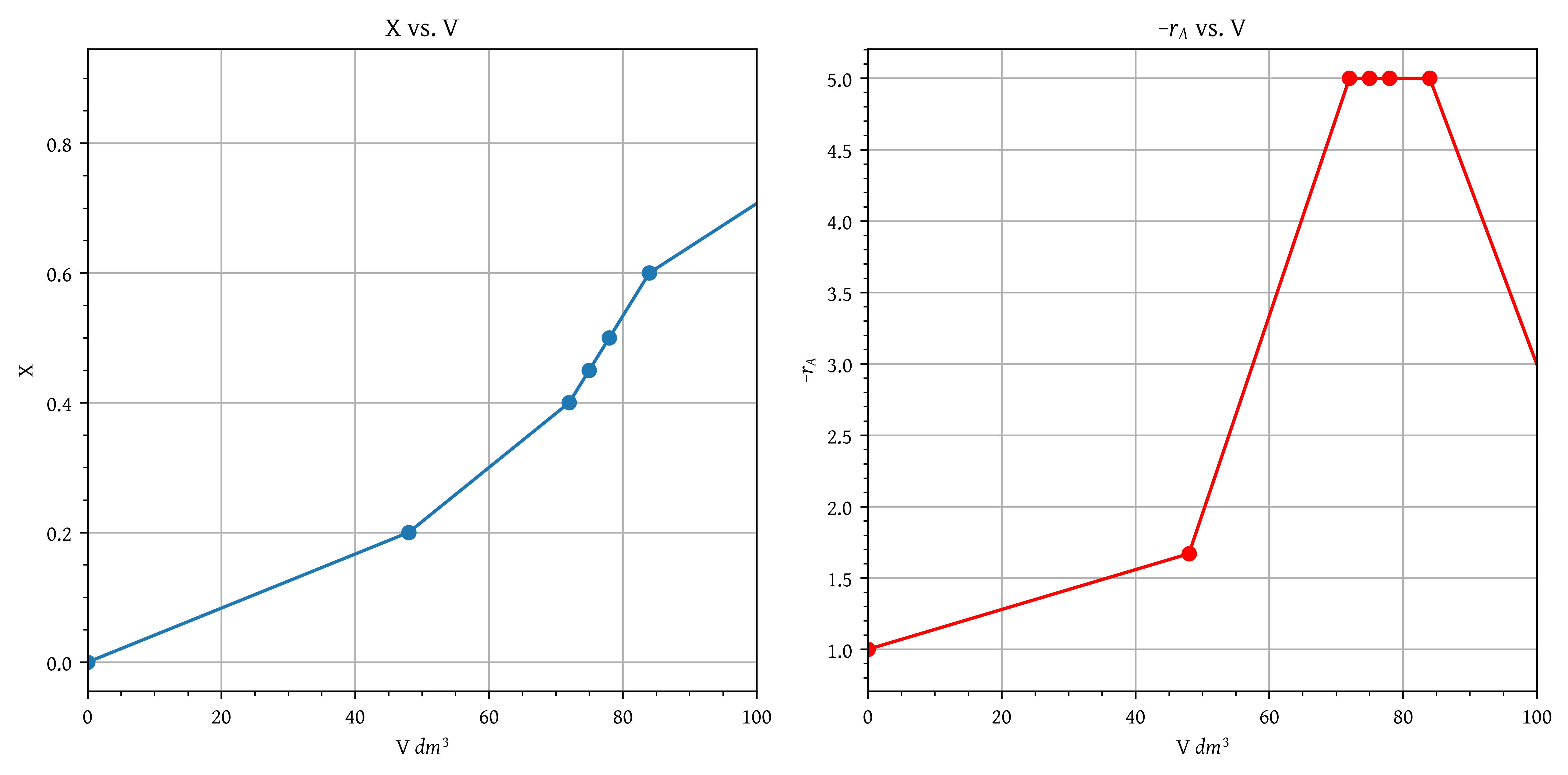
- Plot the conversion and rate of reaction as a function of PFR reactor volume up to a volume of 100 dm^3.
To create this plot (Figure 19), we will need to calculate the volume first for all X as
V = \int_0^x \frac{F_{A0}{-r_A}} dX
This data is given in Table 3
| V (dm^3) | X | -r_A |
|---|---|---|
| 0 | 0 | 1 |
| 48 | 0.2 | 1.67 |
| 72 | 0.4 | 5 |
| 75 | 0.45 | 5 |
| 78 | 0.5 | 5 |
| 84 | 0.6 | 5 |
| 113.978 | 0.8 | 1.25 |
| 142.451 | 0.9 | 0.91 |
Problem 3
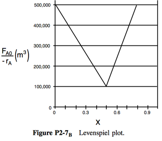
P2-7: The adiabatic exothermic irreversible gas-phase reaction
\ce{2A + B -> 2C}
is to be carried out in a flow reactor for an equimolar feed of A and B. A Levenspiel plot for this reaction is shown in Figure 20 .
- What PFR volume is necessary to achieve 50% conversion?
- What CSTR volume is necessary to achieve 50% conversion?
- What is the volume of a second CSTR added in series to the first CSTR (Part b) necessary to achieve an overall conversion of 80%?
- What PFR volume must be added to the first CSTR (Part b) to raise the conversion to 80%?
- What conversion can be achieved in a 6 \times 10^4 m^3 CSTR? In a 6 \times 10^4 m^3 PFR?
- Think critically to critique the answers (numbers) to this problem.
Solution:
Problem 4
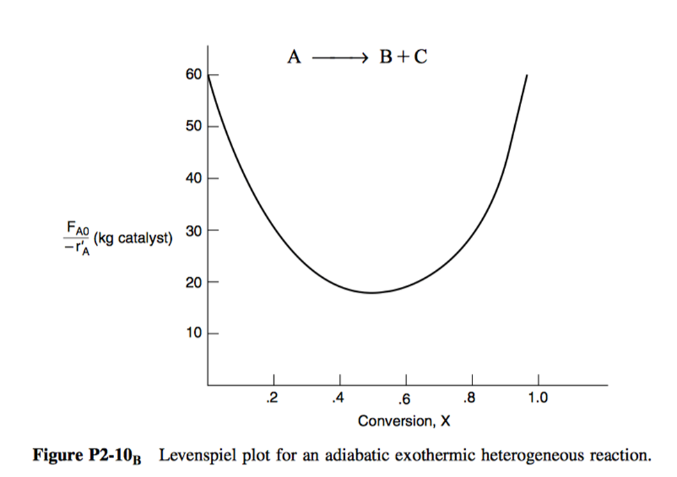
P2.10: The curve shown in Figure 21 is typical of a gas-solid catalytic exothermic reaction carried out adiabatically.
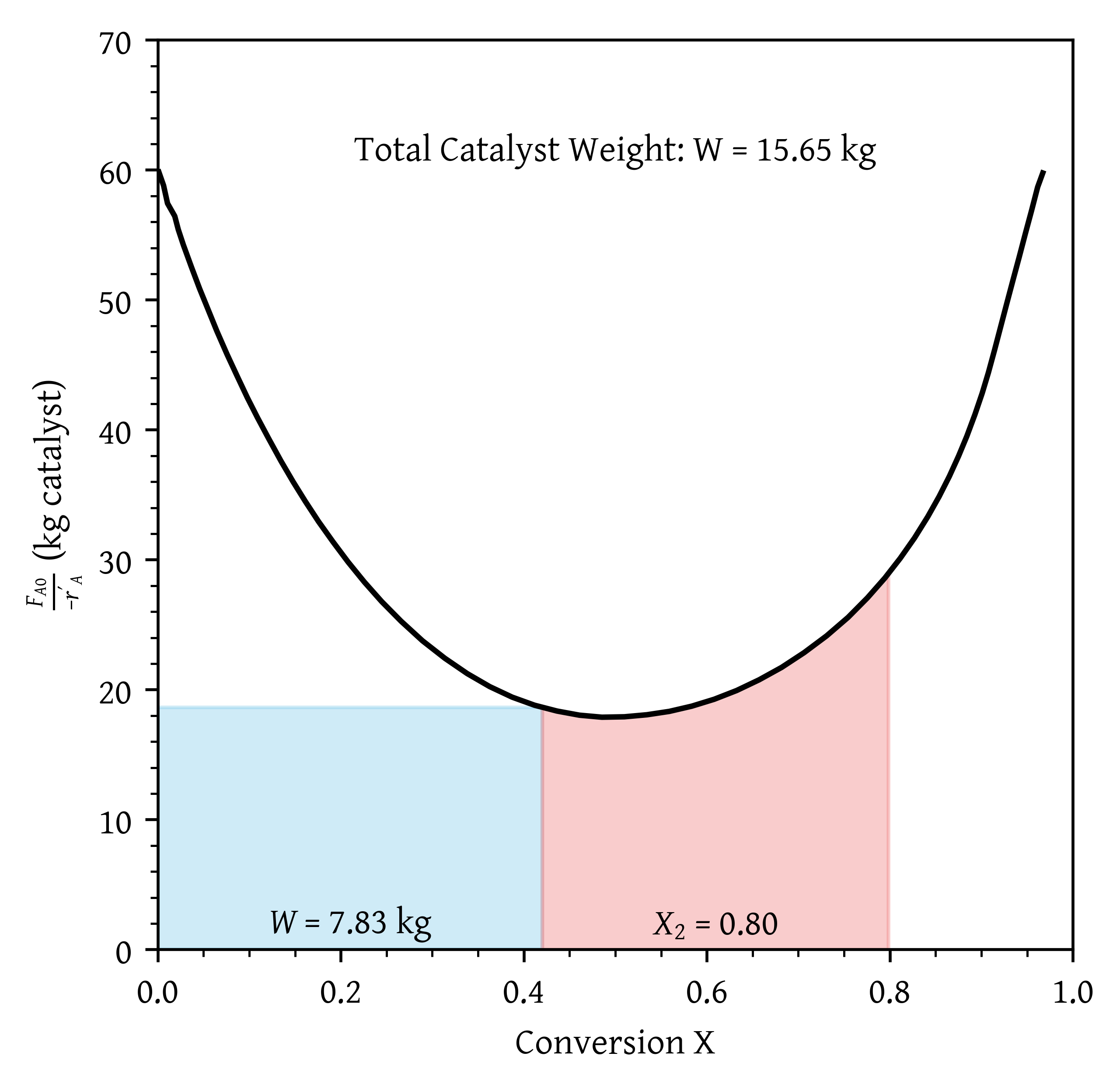
- Assuming that you have a fluidized CSTR and a PBR containing equal weights of catalyst, how should they be arranged for this adiabatic reaction? Use the smallest amount of catalyst weight to achieve 80% conversion of A.
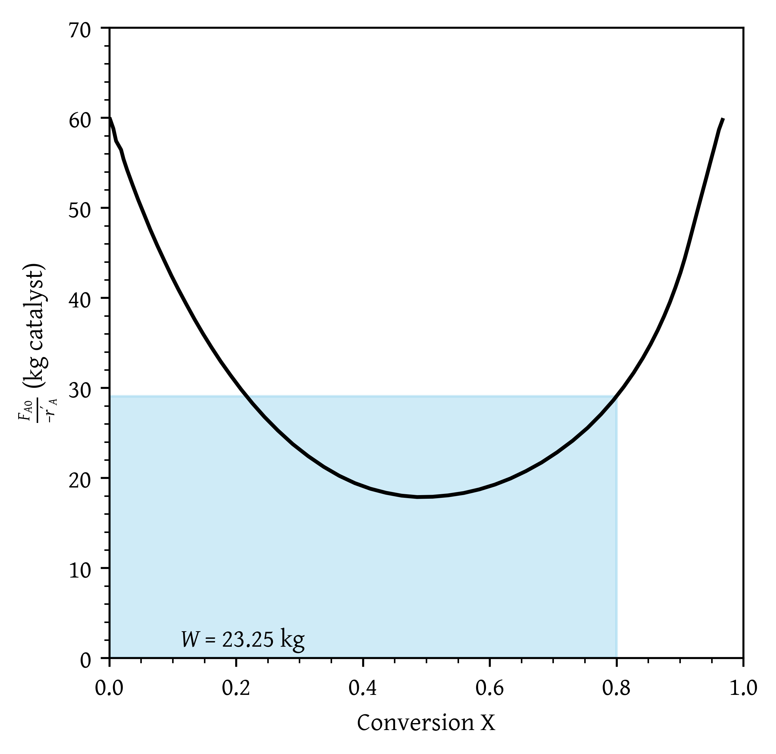
- What is the catalyst weight necessary to achieve 80% conversion in a fluidized CSTR?
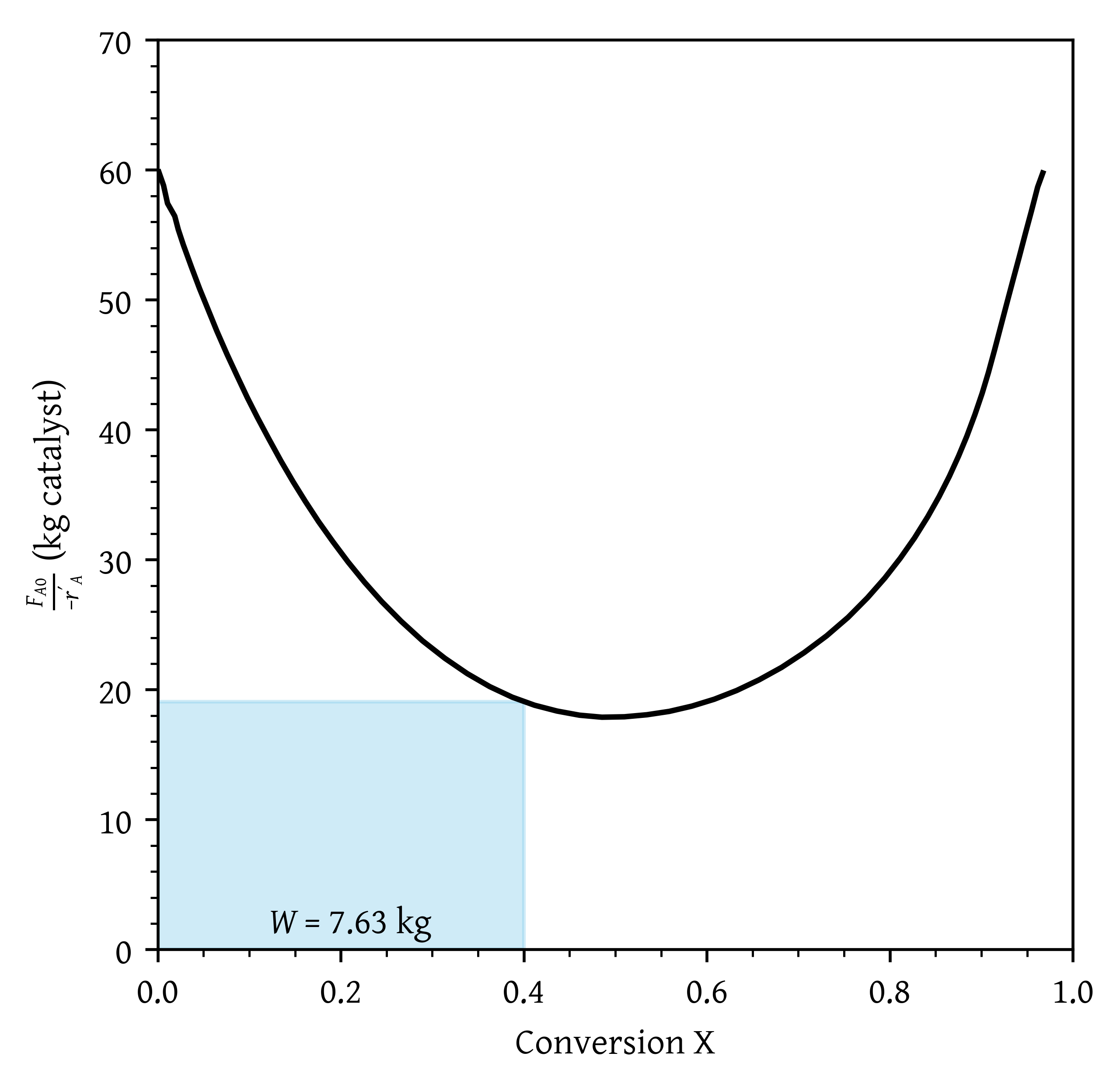
- What fluidized CSTR weight is necessary to achieve 40% conversion?
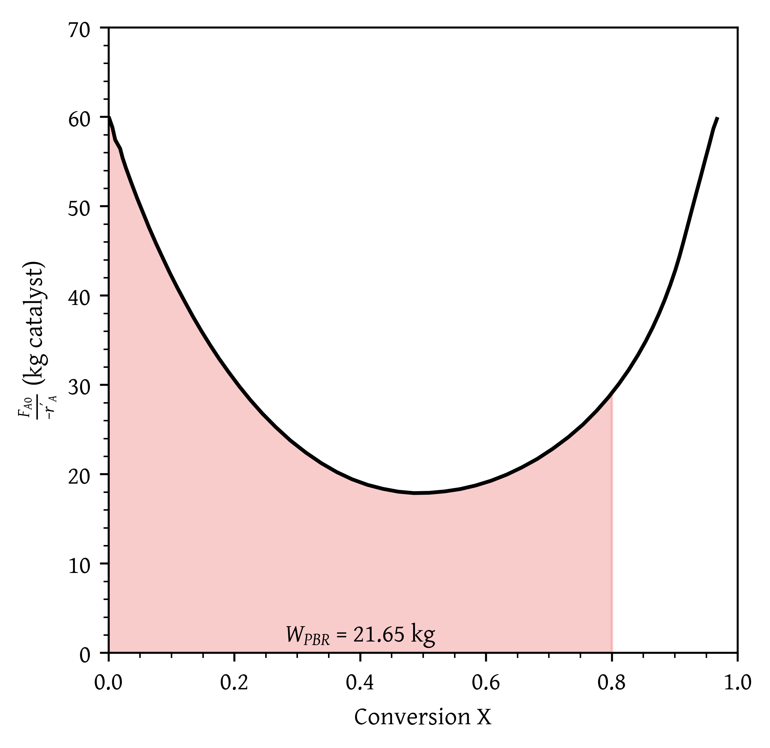
- What PBR weight is necessary to achieve 80% conversion?
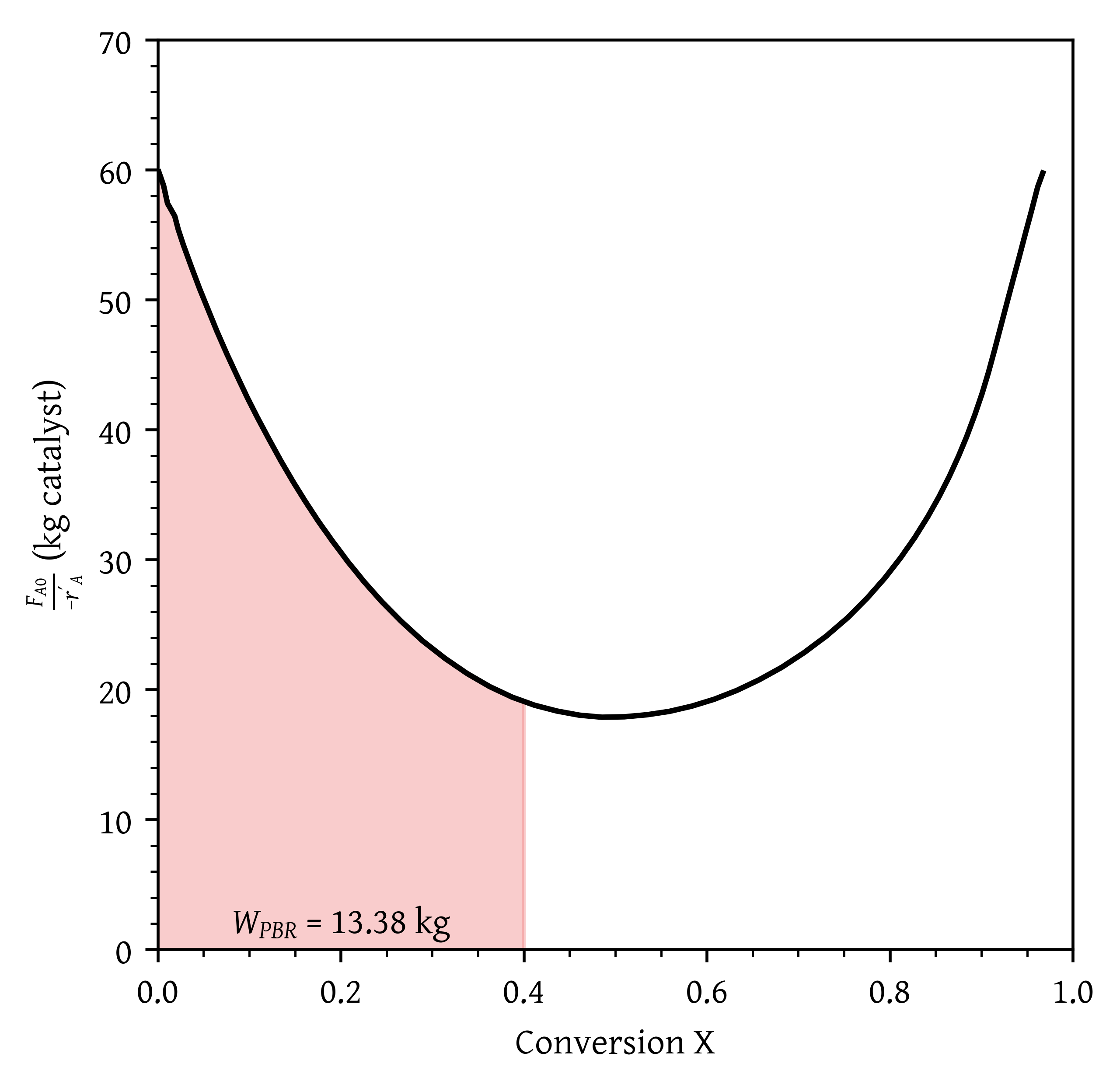
- What PBR weight is necessary to achieve 40% conversion?
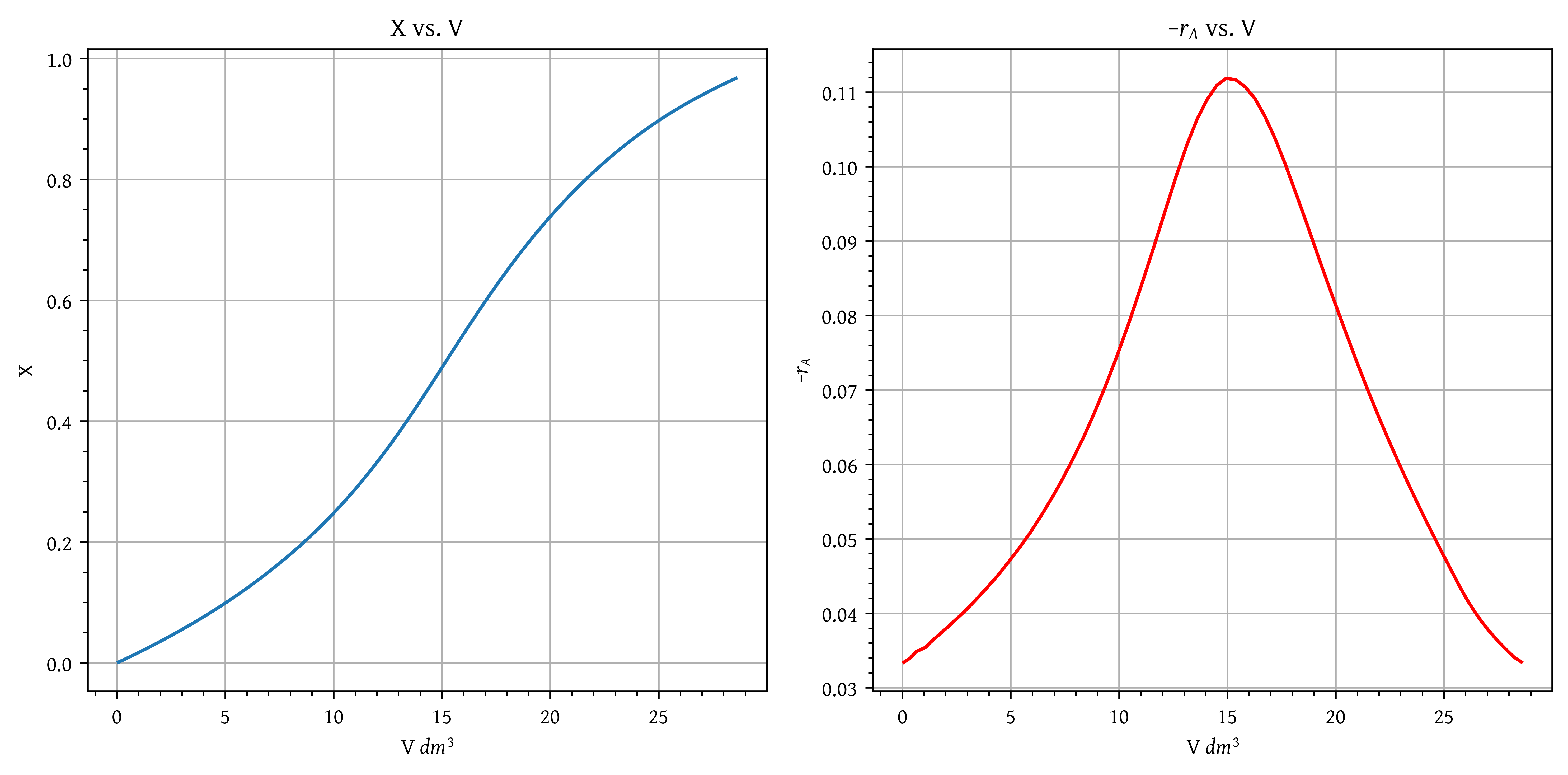
- Plot the rate of reaction and conversion as a function of PBR catalyst weight, W.
Additional information: FA0 = 2 mol/s.
Solution:
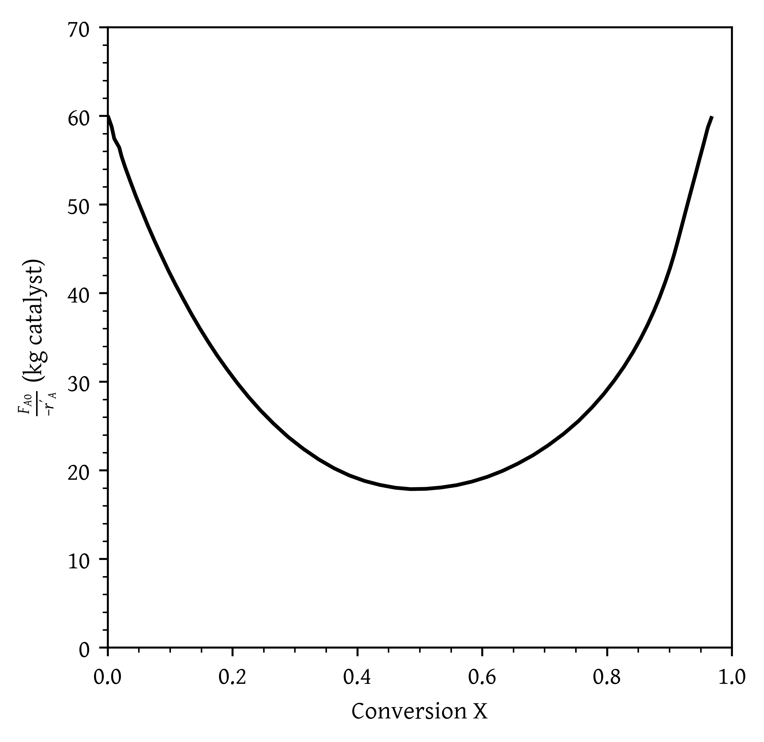
Digitized graph: (Figure 22)
- Assuming that you have a fluidized CSTR and a PBR containing equal weights of catalyst, how should they be arranged for this adiabatic reaction? Use the smallest amount of catalyst weight to achieve 80% conversion of A. (Figure 23)
- What is the catalyst weight necessary to achieve 80% conversion in a fluidized CSTR? (Figure 24)
- What fluidized CSTR weight is necessary to achieve 40% conversion? (Figure 25)
- What PBR weight is necessary to achieve 80% conversion? (Figure 26)
- What PBR weight is necessary to achieve 40% conversion? (Figure 27)
- Plot the rate of reaction and conversion as a function of PBR catalyst weight, W. (Data table: Table 4; Plots: Figure 28)
| V (dm^3) | X | -r_A |
|---|---|---|
| 0.0730885 | 0.00122266 | 0.0334255 |
| 1.597 | 0.02795 | 0.0368764 |
| 3.97751 | 0.0756876 | 0.0436557 |
| 6.4248 | 0.134583 | 0.0531844 |
| 8.88462 | 0.207988 | 0.0670574 |
| 11.6107 | 0.313744 | 0.089225 |
| 14.0622 | 0.436315 | 0.108972 |
| 16.2747 | 0.55899 | 0.109126 |
| 18.6969 | 0.681754 | 0.0921045 |
| 21.4901 | 0.794571 | 0.0699448 |
| 23.7561 | 0.865033 | 0.0549146 |
| 25.4624 | 0.907618 | 0.0450597 |
| 27.1073 | 0.941305 | 0.037535 |
Citation
BibTeX citation:
@online{utikar2024,
  author = {Utikar, Ranjeet},
  title = {Workshop 02 {Solution:} {Conversion} and Reactor Sizing},
  date = {2024-03-03},
  url = {https://cre.smilelab.dev/content/workshops/02-conversion-and-reactor-sizing/solutions.html},
  langid = {en}
}
For attribution, please cite this work as:
Utikar, Ranjeet. 2024. “Workshop 02 Solution: Conversion and
Reactor Sizing.” March 3, 2024. https://cre.smilelab.dev/content/workshops/02-conversion-and-reactor-sizing/solutions.html.