In class activity: Collection and analysis of rate data

Lecture notes for chemical reaction engineering

Determining the Rate Law

The liquid-phase reaction of triphenyl methyl chloride (trityl) (A) and methanol (B)

$$\ce{(C6H5)3CCl + CH3OH -> (C6H5)3COCH3 + HCl}$$

$$\ce{A + B -> C + D}$$

was carried out in a batch reactor at 25°C in a solution of benzene and pyridine in an excess of methanol $C_{B0} = 0.5 \frac{mol}{dm^3}$. (We need to point out that this batch reactor was purchased at the Sunday market in Rijca, Jofostan.) Pyridine reacts with HCl, which then precipitates as pyridine hydro-chloride thereby making the reaction irreversible. The reaction is first order in methanol. The concentration of triphenyl methyl chloride (A) was measured as a function of time and is shown below (Table 1)

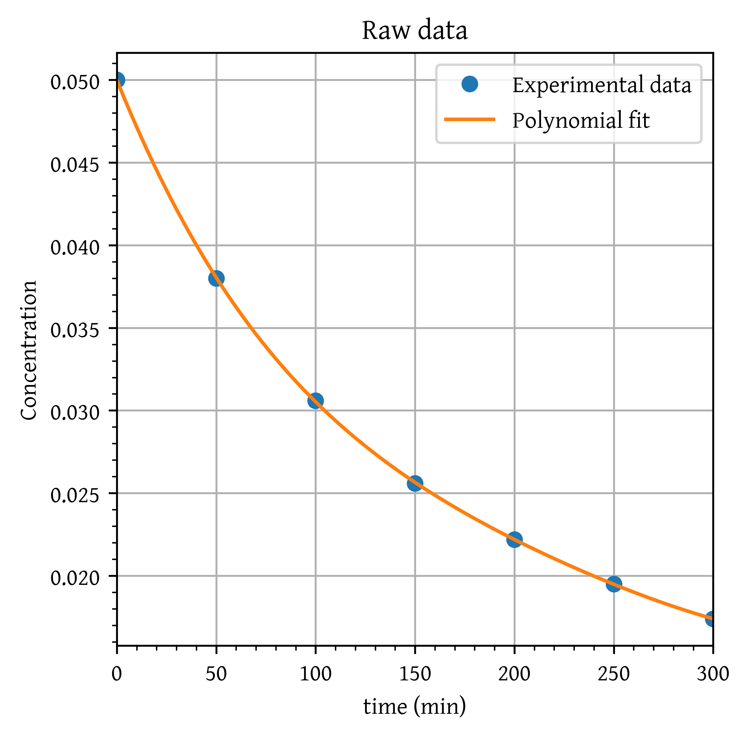
Table 1: Raw data

$t$ (min)	$C_A$ $(mol/dm^3)$
0	0.05
50	0.038
100	0.0306
150	0.0256
200	0.0222
250	0.0195
300	0.0174

1. Determine the reaction order with respect to triphenyl methyl chloride.

2. In a separate set of experiments, the reaction order wrt methanol was found to be first order. Determine the specific reaction-rate constant.

Solution

Part (1) Find the reaction order with respect to trityl.

Step 1 Postulate a rate law.

$$-r_A = k C_A^\alpha C_B^\beta \tag{1}$$

Step 2 Process your data in terms of the measured variable, which in this case is $C_A$.

Step 3 Look for simplifications. Because the concentration of methanol is 10 times the initial concentration of triphenyl methyl chloride, its concentration is essentially constant

$$C_B \approx C_{B0}$$

Substituting for $C_B$ in Equation 1

$$-r_A = k C_{B0}^\beta C_A^\alpha = k' C_A^\alpha$$

Step 4 Apply the CRE algorithm.

Mole Balance

$$\frac{dN_A}{dt} = r_A V$$

Rate Law:

$$-r_A = k' C_A^\alpha$$

Stoichiometry: Liquid $V = V_0$

$$C_A = \frac{N_A}{V_0}$$

Combine: Mole balance, rate law, and stoichiometry

$$-\frac{dC_A}{dt} = k' C_A^\alpha \tag{2}$$

Evaluate: Taking the natural log of both sides of Equation 2

$$\ln \left[ -\frac{dC_A}{dt} \right] = \ln k' + \alpha \ln C_A$$

The slope of a plot of $\ln [-dC_A/dt]$ versus $\ln C_A$ will yield the reaction order α with respect to triphenyl methyl chloride (A)

import numpy as np
from scipy.stats import linregress
import matplotlib.pyplot as plt

# Data
C_B0 = 0.5  # mol/dm^3

t = np.array([0, 50, 100, 150, 200, 250, 300])
C_A = np.array([0.05, 0.038, 0.0306, 0.0256, 0.0222, 0.0195, 0.0174])

C_A0 = C_A[0]

# fit polynomial to the data
coefficients = np.polyfit(t, C_A, deg=4)
polynomial = np.poly1d(coefficients)

t_fit = np.linspace(t.min(), t.max(), 100)
ca_fit = polynomial(t_fit)

plt.plot(t, C_A, 'o', label='Experimental data')
plt.plot(t_fit, ca_fit , '-', label='Polynomial fit')
plt.xlabel('time (min)')
plt.ylabel('Concentration')
plt.title('Raw data')

plt.legend()
plt.grid(True)
plt.xlim(0,300)

plt.show()

# calculate the derivative of the polynomial
dca_dt = np.polyder(polynomial)

ln_ca = np.log(C_A)
ln_dca_dt = np.log(-dca_dt(t))

# fit line
res = linregress(ln_ca, ln_dca_dt)
line = res.slope * ln_ca + res.intercept

plt.plot(ln_ca, ln_dca_dt, 'o', label='Differential analysis')
plt.plot(ln_ca, line, '-', label='fitted line')

plt.annotate(f'Slope = {res.slope:.2e}\nIntercept = {res.intercept:.2f}\n$R^2$ = {res.rvalue**2:.3f}',
             xy=(0.5, 0.15), xycoords='axes fraction', fontsize=12)

plt.xlabel('$\ln C_A$')
plt.ylabel('$\ln(\\frac{-dC_A}{dt})$')

plt.legend()
plt.grid(True)

plt.show()

# pick the closest round order
order = round(res.slope)
a = np.exp(res.intercept)
k = a /C_B0

<>:17: SyntaxWarning: invalid escape sequence '\l'
<>:18: SyntaxWarning: invalid escape sequence '\l'
<>:17: SyntaxWarning: invalid escape sequence '\l'
<>:18: SyntaxWarning: invalid escape sequence '\l'
C:\Users\Ranjeet\AppData\Local\Temp\ipykernel_16332\3516368603.py:17: SyntaxWarning: invalid escape sequence '\l'
  plt.xlabel('$\ln C_A$')
C:\Users\Ranjeet\AppData\Local\Temp\ipykernel_16332\3516368603.py:18: SyntaxWarning: invalid escape sequence '\l'
  plt.ylabel('$\ln(\\frac{-dC_A}{dt})$')

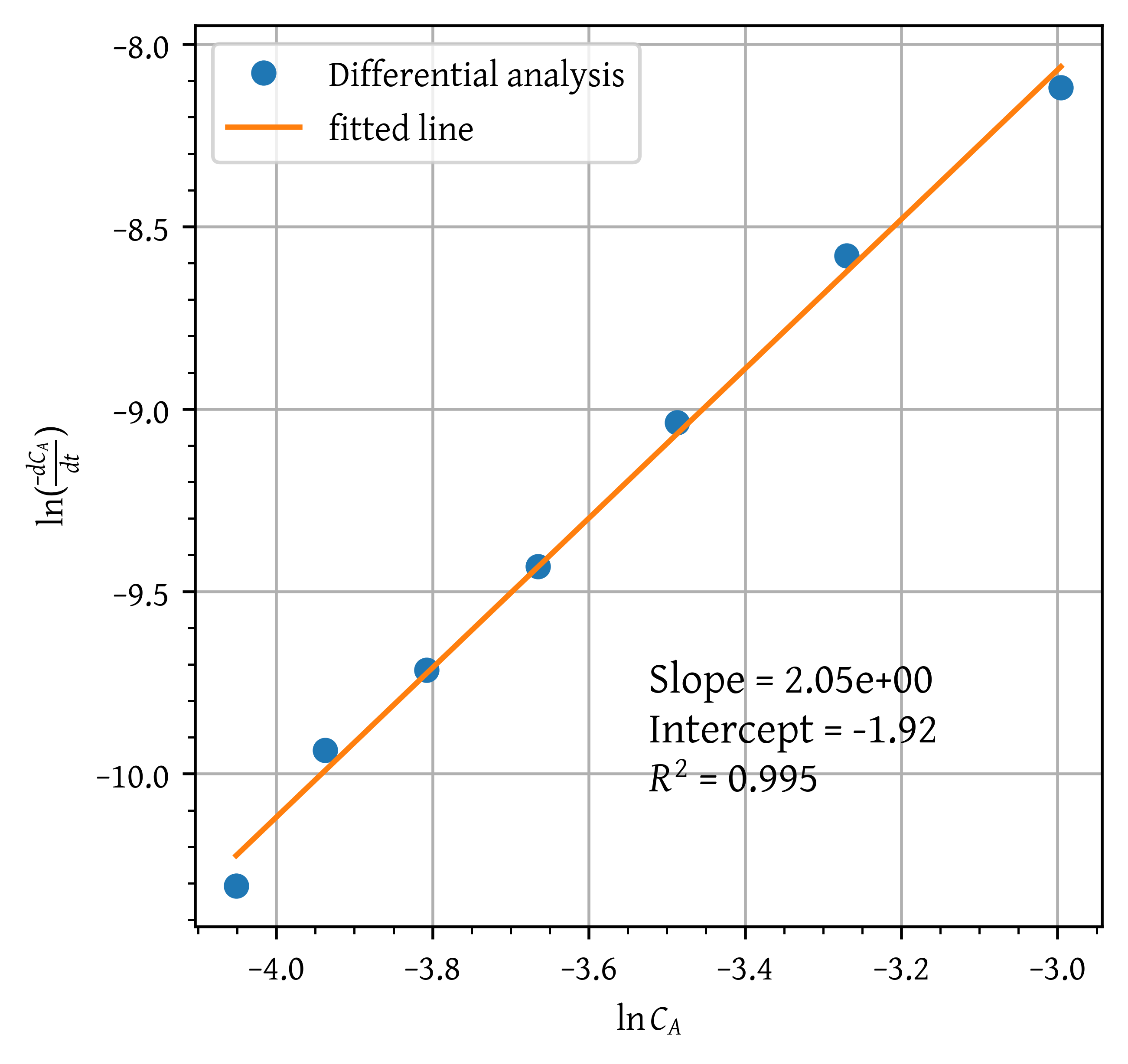
Reaction order is = 2, and $k$ is 0.292 $(dm^3/mol)^2/min$.

Rate law is $-r_A =$ 0.292 $C_A^{2} C_B$

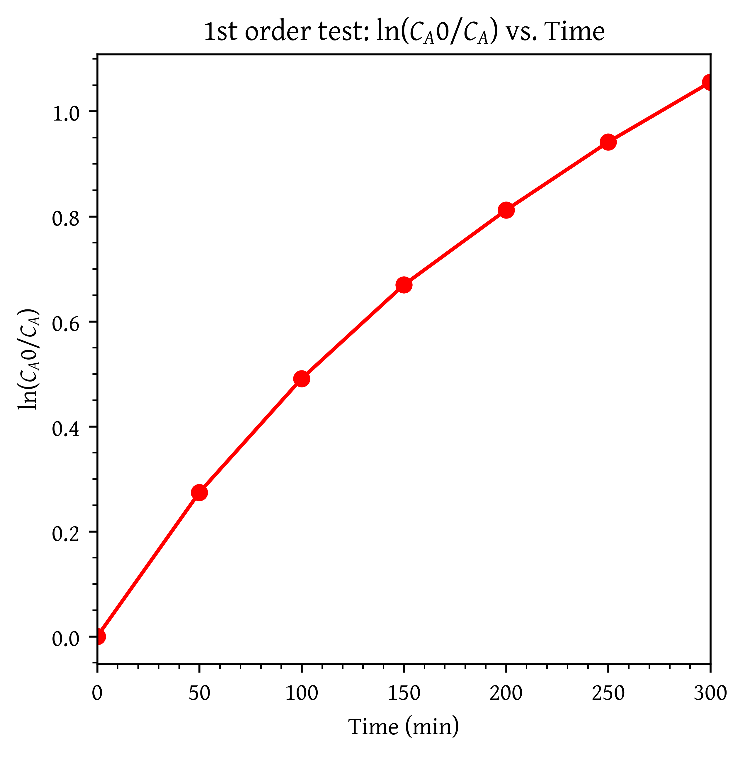
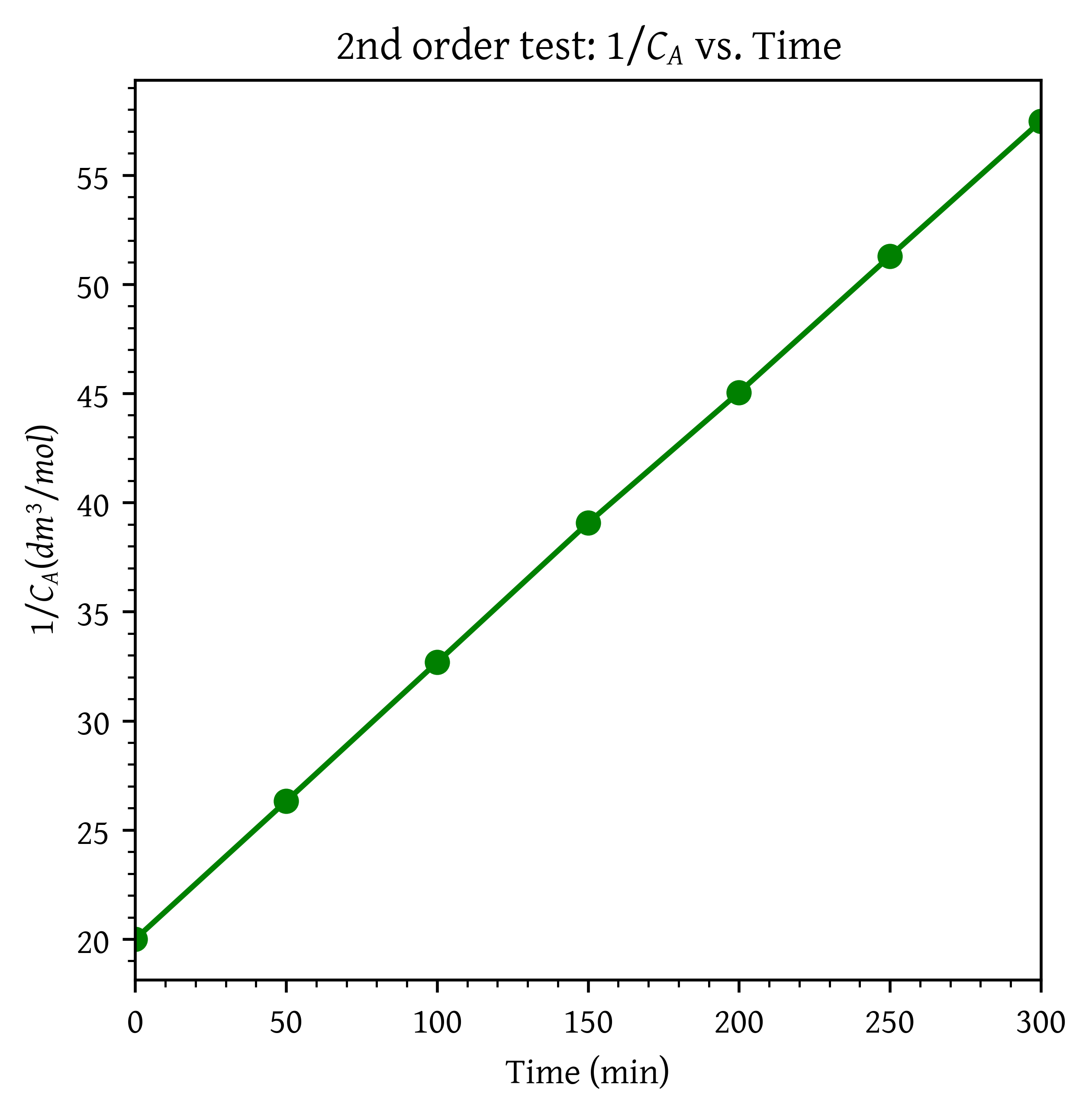
Integral analysis

Use the integral method to confirm that the reaction is second order with regard to triphenyl methyl chloride

Solution

import numpy as np
from scipy.stats import linregress
import matplotlib.pyplot as plt

# Data
C_B0 = 0.5  # mol/dm^3

t = np.array([0, 50, 100, 150, 200, 250, 300])
C_A = np.array([0.05, 0.038, 0.0306, 0.0256, 0.0222, 0.0195, 0.0174])

C_A0 = C_A[0]

ln_ca0_by_ca = np.log(C_A0/C_A)
one_by_ca = 1/C_A

# Plotting

# C_A vs t
plt.plot(t, C_A, 'bo-')
plt.title('0th order test: Concentration of A vs. Time')
plt.xlabel('Time (min)')
plt.ylabel('Concentration of A ($mol/dm^3$)')

plt.xlim(0,300)
plt.show()

# ln(C_A0/C_A) vs t
plt.plot(t, ln_ca0_by_ca, 'ro-')
plt.title('1st order test: $\ln(C_A0/C_A)$ vs. Time')
plt.xlabel('Time (min)')
plt.ylabel('$\ln(C_A0/C_A)$')

plt.xlim(0,300)
plt.show()

# 1/C_A vs t
plt.plot(t, one_by_ca, 'go-')
plt.title('2nd order test: $1/C_A$ vs. Time')
plt.xlabel('Time (min)')
plt.ylabel('$1/C_A (dm^3/mol)$')

plt.xlim(0,300)
plt.show()

<>:29: SyntaxWarning: invalid escape sequence '\l'
<>:31: SyntaxWarning: invalid escape sequence '\l'
<>:29: SyntaxWarning: invalid escape sequence '\l'
<>:31: SyntaxWarning: invalid escape sequence '\l'
C:\Users\Ranjeet\AppData\Local\Temp\ipykernel_16332\965087012.py:29: SyntaxWarning: invalid escape sequence '\l'
  plt.title('1st order test: $\ln(C_A0/C_A)$ vs. Time')
C:\Users\Ranjeet\AppData\Local\Temp\ipykernel_16332\965087012.py:31: SyntaxWarning: invalid escape sequence '\l'
  plt.ylabel('$\ln(C_A0/C_A)$')

As the plot of $1/C_A$ vs. t is linear, the reaction is second order with respect to A.

Use of Regression to Find the Rate-Law Parameters

Use polynomial regression to estimate rate equation. Assume the reaction order is not 1.

Solution

For constant volume batch reactor,

$$\frac{dC_A}{dt} = -k' C_A^\alpha$$

and integrating with the initial condition when $t = 0$ and $C_A = C_{A0}$ for $\alpha \neq 1.0$ gives us:

$$t = \frac{1}{k'} \left[ \frac{C_{A0}^{(1-\alpha)} - C_A^{(1-\alpha)}}{1-\alpha} \right]$$

We want to minimize $s^2$ to give $\alpha$ and $k'$.

$$s^2 = \sum_{i=1}^{N} (t_{im} - t_{ic})^2$$

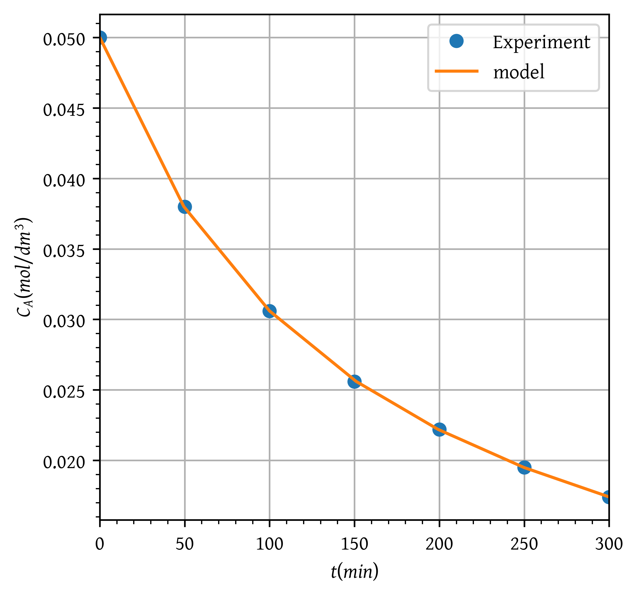
import numpy as np
import matplotlib.pyplot as plt
from scipy.optimize import minimize

# Data
C_B0 = 0.5  # mol/dm^3

t = np.array([0, 50, 100, 150, 200, 250, 300])
C_A = np.array([0.05, 0.038, 0.0306, 0.0256, 0.0222, 0.0195, 0.0174])

C_A0 = C_A[0]

# Initial guesses of k and n

# here k is the clubbed constant k * C_B0
k = 1 
n = 0

# Objective function to minimize: the difference between t (experimental) and t (model)

def objective(params):
   k, n = params

   # Calculate t model

   t_model = (1/k) * (C_A0**(1-n) - C_A**(1-n))/ (1-n)
   ssr = np.sum((t - t_model)**2)  # Sum of squared residuals
   return ssr

# Minimize the objective function
result = minimize(objective, [k,n], bounds=[(1e-4, 1e4), (0, 5)])

# Extract the results
k_opt, n_opt = result.x
success = result.success

# Check if the solution was successful
if not success:
    print("Optimization was not successful. Try different initial guesses or methods.")

# final evaluation
t_model = (1/k_opt) * (C_A0**(1-n_opt) - C_A**(1-n_opt))/ (1-n_opt)

# plot the data
plt.plot(t, C_A, 'o', label='Experiment')
plt.plot(t_model, C_A, '-', label='model')
plt.xlabel('$t (min)$')
plt.ylabel('$C_A (mol/dm^3)$')

plt.legend()
plt.grid(True)
plt.xlim(min(t),max(t))

plt.show()

Initial guess for Reaction order is = 0.00, and $k$ is 1.000e+00.

Optimized value of Reaction order is = 2.04, and $k$ is 2.934e-01.

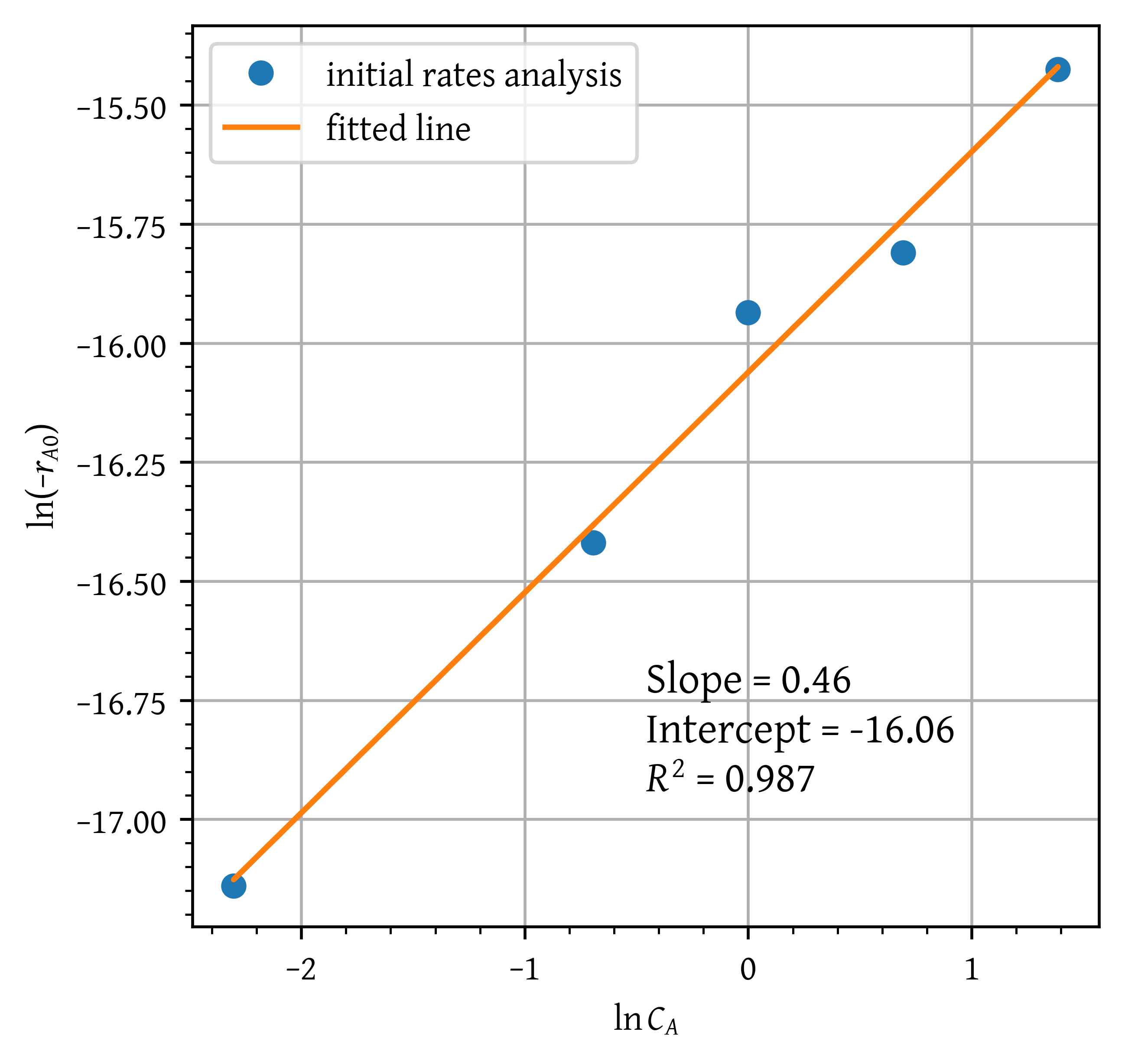
Method of initial rates

The dissolution of dolomite using hydrochloric acid:

$$\ce{4HCl + CaMg(CO3)2 -> Mg^2+ + Ca^2+ + 4Cl- + 2CO2 + 2H2O}$$

Concentration of HCl at various times was determined from atomic absorption spectrophotometer measurements of the $\ce{Ca^2+}$ and $\ce{Mg^2+}$ ions (Table 2). Determine the rate constant and order of reaction.

Table 2: HCL concentration

$C_{HCl,0}$ (N)	Initial reaction rate $-r_{HCl,0}$ ($mol/cm^2 s \times 10^7$)
1	1.2
4	2.0
2	1.36
0.1	0.36
0.5	0.74

Solution

The mole balance for constant V batch reactor at t = 0:

$$\left( \frac{-dC_{HCl}}{dt}\right)_0 = -(r_{HCl})_0 = k C_{HCl,0}^\alpha$$

Taking log $$\ln \left( \frac{-dC_{HCl}}{dt}\right)_0 = \ln k \alpha \ln C_{HCl,0}$$

import numpy as np
from scipy.stats import linregress
import matplotlib.pyplot as plt

ca0 = np.array([1, 4, 2, 0.1, 0.5])
ra0 = np.array([1.2, 2.0, 1.36, 0.36, 0.74]) * 1e-7

ln_ca0 = np.log(ca0)
ln_ra0 = np.log(ra0)

# fit line
res = linregress(ln_ca0, ln_ra0)
line = res.slope * ln_ca0 + res.intercept

plt.plot(ln_ca0, ln_ra0, 'o', label='initial rates analysis')
plt.plot(ln_ca0, line, '-', label='fitted line')

plt.annotate(f'Slope = {res.slope:.2f}\nIntercept = {res.intercept:.2f}\n$R^2$ = {res.rvalue**2:.3f}',
             xy=(0.5, 0.15), xycoords='axes fraction', fontsize=12)

plt.xlabel('$\ln C_A$')
plt.ylabel('$\ln(-r_{A0})$')

plt.legend()
plt.grid(True)

plt.show()

order = res.slope
k = np.exp(res.intercept)

<>:21: SyntaxWarning: invalid escape sequence '\l'
<>:22: SyntaxWarning: invalid escape sequence '\l'
<>:21: SyntaxWarning: invalid escape sequence '\l'
<>:22: SyntaxWarning: invalid escape sequence '\l'
C:\Users\Ranjeet\AppData\Local\Temp\ipykernel_16332\399930876.py:21: SyntaxWarning: invalid escape sequence '\l'
  plt.xlabel('$\ln C_A$')
C:\Users\Ranjeet\AppData\Local\Temp\ipykernel_16332\399930876.py:22: SyntaxWarning: invalid escape sequence '\l'
  plt.ylabel('$\ln(-r_{A0})$')

Reaction order is = 0.46, and $k$ is 1.058e-07.

Using a Differential Reactor to Obtain Catalytic Rate Data

The formation of methane from carbon monoxide and hydrogen using a nickel catalyst was studied by Pursley. The reaction

$$\ce{3H2 + CO ->[Ni] CH4 + H2O}$$

was carried out at 500 °F in a differential reactor where the effluent concentration of methane was measured. The raw data is shown in Table 3

Table 3: Raw data

Run	$P_{CO}$ (atm)	$P_{H_2}$ (atm)	$C_{CH_4}$ $(mol/dm^3) \times 10^{4}$
1	1	1.0	1.73
2	1.8	1.0	4.40
3	4.08	1.0	10.0
4	1.0	0.1	1.65
5	1.0	0.5	2.47
6	1.0	4.0	1.75

The exit volumetric flow rate from a differential packed bed containing 10 g of catalyst was maintained at 300 $dm^3/min$ for each run. The partial pressures of $\ce{H2}$ and $\ce{CO}$ were determined at the entrance to the reactor, and the methane concentration was measured at the reactor exit. Determine the rate law and rate law parameters.

Solution

• Reaction temperature: 500°F (isothermal reaction)
• Weight of catalyst : ΔW = 10 g
• Exit volumetric flow rate v = 300 $dm^3/min$

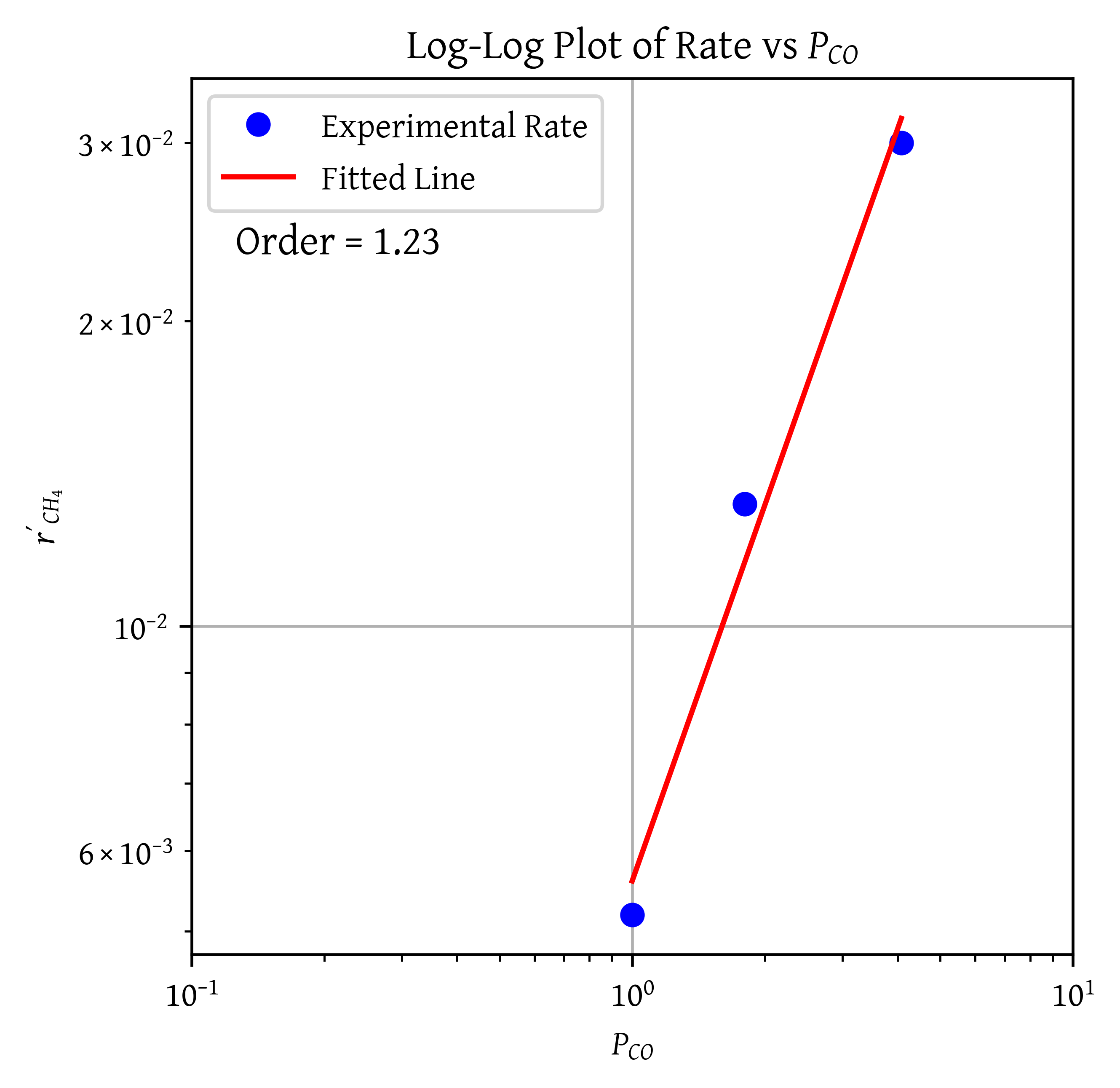
The reaction-rate law is assumed to be the product of a function of the partial pressure of $\ce{CO}$ and a function of the partial pressure of $\ce{H2}$,

$$r'_{CH_4} = f(CO) \times g(H_2)$$

For the first 3 experiments, $P_{H_2}$ is constant. We use this data to determine the dependence on $P_{CO}$.

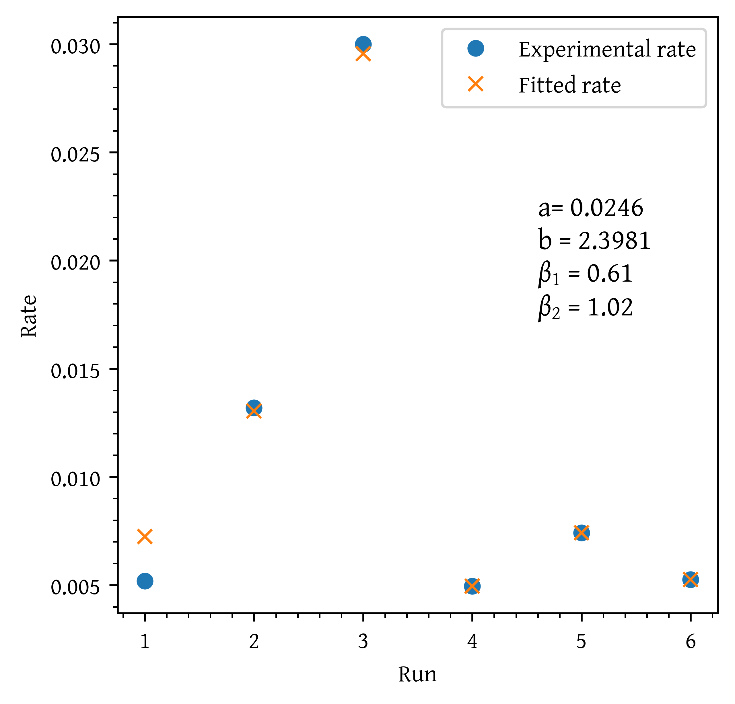
For the experiments 1, 4, 5, 6, $P_{CO}$ is constant. We use this data to determine the dependence on $P_{H_2}$

The rate in a differential reactor is given by

$$-r'_A = \frac{F_p}{\Delta W}$$

$$-r'_{CO} = r'_{CH_4} = \frac{F_{CH_4}}{\Delta W}$$

For constant $H_2$ partial pressure,

$$r'_{CH_4} = k' P_{CO}^\alpha$$

Taking log $$\ln (r'_{CH_4}) = \ln k' + \alpha \ln P_{CO}$$

For constant $CO$ partial pressure,

$$r'_{CH_4} = g(H_2)$$

From the data:

At low $H_2$ partial pressures, where $r'_{CH_4}$ increases as $P_{H_2}$ increases, the rate law may be of the form

$$r'_{CH_4} \propto P_{H_2}^{\beta_1} \tag{3}$$

At high $H_2$ partial pressures,where $r'_{CH_4}$ decreases as $P_{H_2}$ increases, the rate law may be of the form

$$r'_{CH_4} \propto \frac{1}{P_{H_2}^{\beta_2}} \tag{4}$$

Combining Equation 3, and Equation 4 we can write

$$r'_{CH_4} \propto \frac{P_{H_2}^{\beta_1}}{1 + b P_{H_2}^{\beta_2}} \tag{5}$$

And the overall rate equation becomes:

$$r'_{CH_4} = \frac{a P_{CO}^\alpha P_{H_2}^{\beta_1}}{1 + b P_{H_2}^{\beta_2}} \tag{6}$$

We can use regression to calculate estimate $\beta_1$, $\beta_2$, and constants a, and b.

import numpy as np
from numpy.lib import recfunctions as rfn
from scipy.stats import linregress
import matplotlib.pyplot as plt

Temperature = 500  # deg. F
DeltaW = 10 # g
V_0 = 300   # dm^3/min

dtype = [('Run', int), ('P_CO', float), ('P_H2', float), ('C_CH4', float)]
data = np.array([
    (1, 1.0, 1.0, 1.73e-4),
    (2, 1.8, 1.0, 4.40e-4),
    (3, 4.08, 1.0, 10.0e-4),
    (4, 1.0, 0.1, 1.65e-4),
    (5, 1.0, 0.5, 2.47e-4),
    (6, 1.0, 4.0, 1.75e-4)
], dtype=dtype)

pco = data["P_CO"]
ph2 = data["P_H2"]
cch4 = data["C_CH4"]

rate = V_0 * cch4 / DeltaW 

data = rfn.append_fields(data, 'Rate', rate, usemask=False)

# Use first three points to estimate alpha

pco_a = pco[:3]
rate_a = rate[:3]

ln_pco_a = np.log(pco_a)
ln_rate_a= np.log(rate_a)

# fit line
res = linregress(ln_pco_a, ln_rate_a)
line = res.slope * ln_pco_a + res.intercept

alpha = res.slope

plt.loglog(pco_a, rate_a, 'bo', label='Experimental Rate')  # Original data on log-log scale
plt.loglog(pco_a, np.exp(line), 'r-', label='Fitted Line')  # Convert the log of the fitted line back with exp

plt.xlabel('$P_{CO}$')
plt.ylabel('$r\'_{CH_4}$')
plt.title('Log-Log Plot of Rate vs $P_{CO}$')
plt.legend()
plt.grid(True)
plt.xlim(0.1, 10)

plt.annotate(f'Order = {alpha:.2f}', xy=(0.05, 0.8), xycoords='axes fraction', fontsize=12)

plt.show()

Reaction order with respect to $CO$ is $\alpha =$ 1.23.

Had we included more points, we would have found that the reaction is essentially first order.

We now use data from all the runs to estimate other parameters of the rate expression

$$r'_{CH_4} = \frac{a P_{CO} P_{H_2}^{\beta_1}}{1 + b P_{H_2}^{\beta_2}} \tag{7}$$

import numpy as np
import matplotlib.pyplot as plt
from scipy.optimize import least_squares

# Objective function to minimize: the difference between rate (experimental) and rate (calculated)
def objective(params, *args):

   a, b, beta_1, beta_2  = params
   pco, ph2,rate_obs = args

   # calculate rate
   rate_c = (a * pco * ph2**beta_1)/ (1 + b * ph2**beta_2)
   return rate_obs - rate_c

# Initial guesses
a = 1 
b = 1
beta_1 = 1 
beta_2 = 1

guess = np.array([a,b,beta_1,beta_2])
bounds = (
   [1e-3, 1e-3, 0, 0],  # lower bound
   [1e3, 1e3, 3, 3]     # upper bound
)
args = (pco, ph2, rate)

# Minimize the objective function
result = least_squares(objective, guess, args=args, bounds=bounds)

# Extract the results
# Results from Fogler 5e
# a_opt = 0.0252715
# b_opt = 2.4872569
# beta_1_opt = 0.616542
# beta_2_opt = 1.0262047

a_opt, b_opt, beta_1_opt, beta_2_opt = result.x
rate_c = (a_opt * pco * ph2**beta_1_opt)/ (1 + b_opt * ph2**beta_2_opt)

# plot the data
plt.plot(data["Run"], rate, 'o', label='Experimental rate')
plt.plot(data["Run"], rate_c, 'x', label='Fitted rate')

plt.annotate(
    f'a= {a_opt:.4f}\n'\
    f'b = {b_opt:.4f}\n'\
    f'$\\beta_1$ = {beta_1_opt:.2f}\n'\
    f'$\\beta_2$ = {beta_2_opt:.2f}',
    xy=(0.7, 0.5), 
    xycoords='axes fraction',
    fontsize=12
)

plt.xlabel('Run')
plt.ylabel('Rate')

plt.legend()

plt.show()

The final constants are:

a = 0.0246

b = 2.3981

$\beta_1$ = 0.61

$\beta_2$ = 1.02

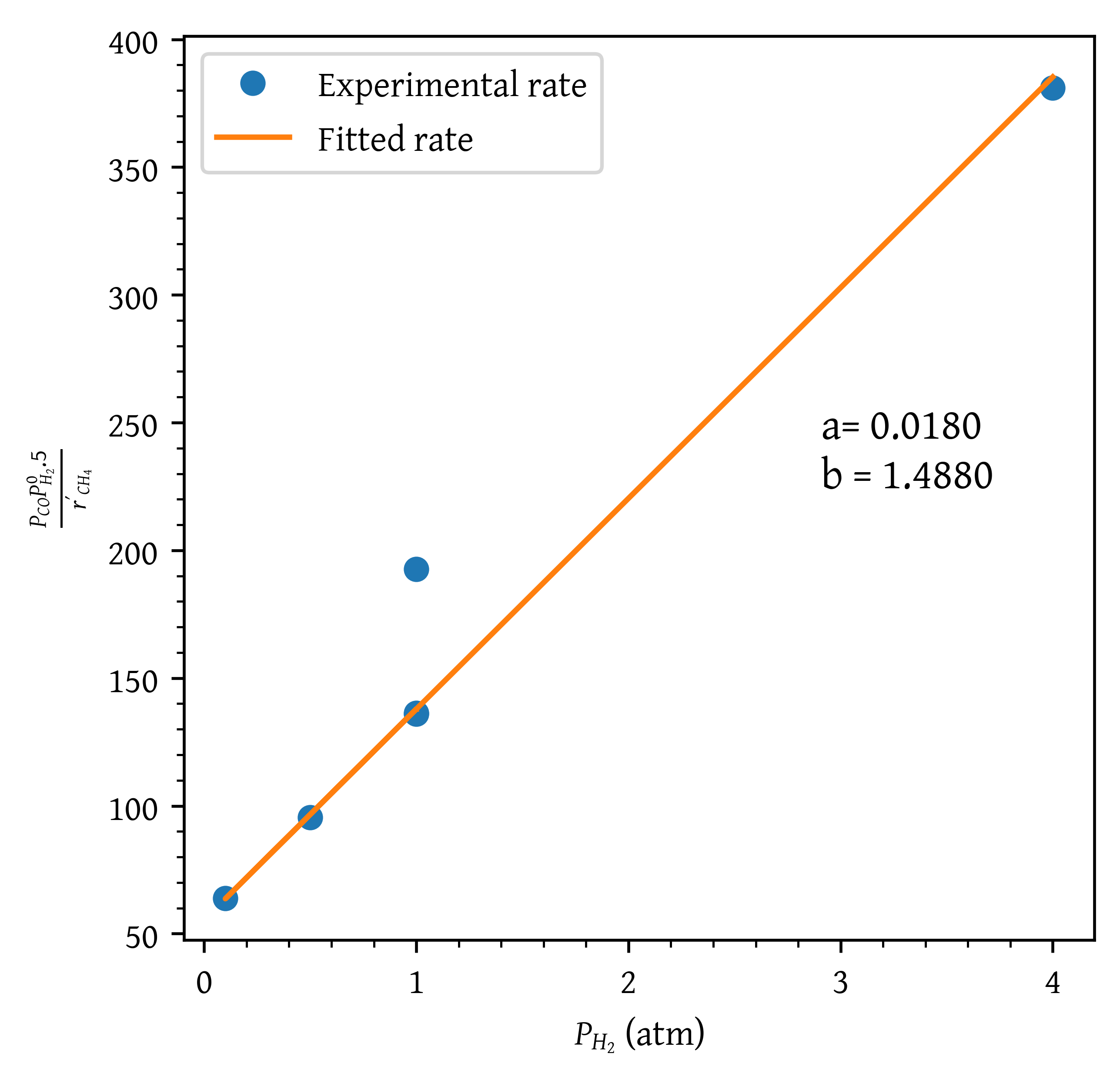
If we assume hydrogen undergoes dissociative adsorption on the catalyst surface, we would expect a dependence on the partial pressure of hydrogen to be to the $1/2$ power. Because 0.61 is close to 0.5, we are going to regress the data again, setting $\beta_1 = 1/2$ and $\beta_2$ = 1.0.

# Objective function to minimize: the difference between rate (experimental) and rate (calculated)
def objective2(params, *args):

   a, b = params
   pco, ph2,rate_obs = args

   # calculate rate
   rate_c = (a * pco * ph2**0.5)/ (1 + b * ph2)
   return rate_obs - rate_c

# Initial guesses
a = 1 
b = 1

guess = np.array([a,b])
bounds = (
   [1e-3, 1e-3],  # lower bound
   [1e3, 1e3]     # upper bound
)
args = (pco, ph2, rate)

# Minimize the objective function
result = least_squares(objective2, guess, args=args, bounds=bounds)

# Extract the results
# Results from Fogler 5e
# a_opt = 0.018
# b_opt = 1.49

a_opt, b_opt = result.x
rate_c = (a_opt * pco * ph2**0.5)/ (1 + b_opt * ph2)

lin_e = pco*ph2**0.5/rate
lin_c = pco*ph2**0.5/rate_c

# plot the data
plt.plot(ph2, lin_e, 'o', label='Experimental rate')
plt.plot(ph2, lin_c, '-', label='Fitted rate')

plt.annotate(
    f'a= {a_opt:.4f}\n'\
    f'b = {b_opt:.4f}',
    xy=(0.7, 0.5), 
    xycoords='axes fraction',
    fontsize=12
)

plt.xlabel('$P_{H_2}$ (atm)')
plt.ylabel('$\\frac{P_{CO} P_{H_2}^0.5}{r\'_{CH_4}}$')

plt.legend()

plt.show()

The final constants are:

a = 0.0180

b = 1.4880