import numpy as np
import matplotlib.pyplot as plt
from scipy.integrate import solve_ivp

# Constants
R = 8.314 # J/mol K
TR = 273 # K

# A -> B + C
# 0: A; 1: B; 2: C

HF = np.array ([-70.0, -50.0, -40.])*1000   # J/mol
CP = np.array ([40.0, 25.0, 15.0]) # J/mol K

E = 31.4 * 1e3 # J/mol
k = lambda t: 0.133 * np.exp( (E/R) * (1/450.0 - 1/t) ) # dm3/ kgcat s

def pfr (w, x, *args):
  X = x[0]
  (ca0, fa0, T0, epsilon, delta_hr_tr, delta_cp, theta) = args

  # Calculate T using energy balance
  T  = T0 + X * (-delta_hr_tr)/( np.sum(theta * CP) + X * delta_cp)
  ca = ca0 * (( 1 - X ) / ( 1 + epsilon * X )) * (T0/T)

  rate = k(T) * ca # -r_A
  dxdw = rate/fa0

  return [dxdw]

# Data
nu = np.array ([-1.0, 1.0, 1.0]) # stoichiometric coefficients

V_0 = 20 # dm3/s
P0 = 10 # atm
T0 = 450 # K

fa0 = P0 * V_0/ (R * T0)
ca0 = fa0/V_0

# inlet mole fraction
y0 = np.array ([1.0, 0.0, 0.0])
theta = np.array([1.0, 0.0, 0.0])

# Heat of reaction at 298K
delta_hr_tr = np.sum(HF * nu)
delta_cp = np.sum(CP * nu)

ya0 = y0[0]
epsilon = ya0 * np.sum(nu)


args = (ca0, fa0, T0, epsilon, delta_hr_tr, delta_cp, theta)

# initial condition
initial_conditions = np.array([0])
w_final = 50 # kg

sol = solve_ivp(pfr,
                [0, w_final],
                initial_conditions,
                args=args,
                dense_output=True)

w = np.linspace(0,w_final, 1000)
x = sol.sol(w)[0]
T = T0 + x * (-delta_hr_tr)/( np.sum(theta * CP) + x * delta_cp)Solutions to workshop 07: Non-isothermal reactor design
Lecture notes for chemical reaction engineering
Try following problems from Fogler 5e P 11-5, P 11-6, P 12-6, P 12-21
We will go through some of these problems in the workshop.
P 11-5
The elementary, irreversible gas-phase reaction
\ce{ A -> B + C }
is carried out adiabatically in a PFR packed with a catalyst. Pure A enters the reactor at a volumetric flow rate of 20 dm3/s, at a pressure of 10 atm, and a temperature of 450 K.
Additional information:
C_{P_A} = 40 J/mol \cdot K; C_{P_B} = 25 J/mol \cdot K; C_{P_C} = 15 J/mol \cdot K
H_A^{\circ} = -70 kJ/mol; H_B^{\circ} = -50 kJ/mol; H_C^{\circ} = -40 kJ/mol
All heats of formation are referenced to 273 K.
k = 0.133 \exp \left[ \frac{E}{R} \left( \frac{1}{450} - \frac{1}{T} \right) \right] \; \frac{dm^3}{kg-cat \cdot s} \; \text{with} \, E = 31.4 kJ/mol
Plot and then analyze the conversion and temperature down the plug-flow reactor until an 80% conversion (if possible) is reached. (The maximum catalyst weight that can be packed into the PFR is 50 kg.) Assume that \Delta P = 0.0.
Vary the inlet temperature and describe what you find.
Plot the heat that must be removed along the reactor ( Q vs. V) to maintain isothermal operation.
Now take the pressure drop into account in the PBR with \rho_b = 1 kg/dm^3. The reactor can be packed with one of two particle sizes. Choose one.
\alpha = 0.019/kg-cat \: \text{for particle diameter} \: D_1 \alpha = 0.0075/kg-cat \: \text{for particle diameter} \: D_2
- Plot and then analyze the temperature, conversion, and pressure along the length of the reactor. Vary the parameters \alpha and P_0 to learn the ranges of values in which they dramatically affect the conversion.
Solution
| Parameter | Value |
|---|---|
| T_R | 273.00 K |
| P_0 | 10.00 bar |
| \Delta H^\circ_{Rx} (T_R) | -20000.00 J/mol |
| \Delta C_P | 0.00 J/mol\ K |
| \epsilon | 1.00 |
| C_{A0} | 2.673e-03 mol/dm^3 |
| F_{A0} | 0.053 mol/s |
Energy balance:
T = 450.00 + 500.00 X
Catalyst weight required to achieve 80% conversion: 43.14 kg
Temperature at 80% conversion: 850.18 K
Exit (W = 50.00 kg) conversion: 0.91
Exit (W = 50.00 kg) temperature: 903.19 K
plt.plot(w,x, label="Conversion")

plt.xlim(0,50)
plt.ylim(0,1)
plt.grid()
plt.legend()

plt.xlabel('Catalyst weight ($kg$)')
plt.ylabel('Conversion')

plt.show()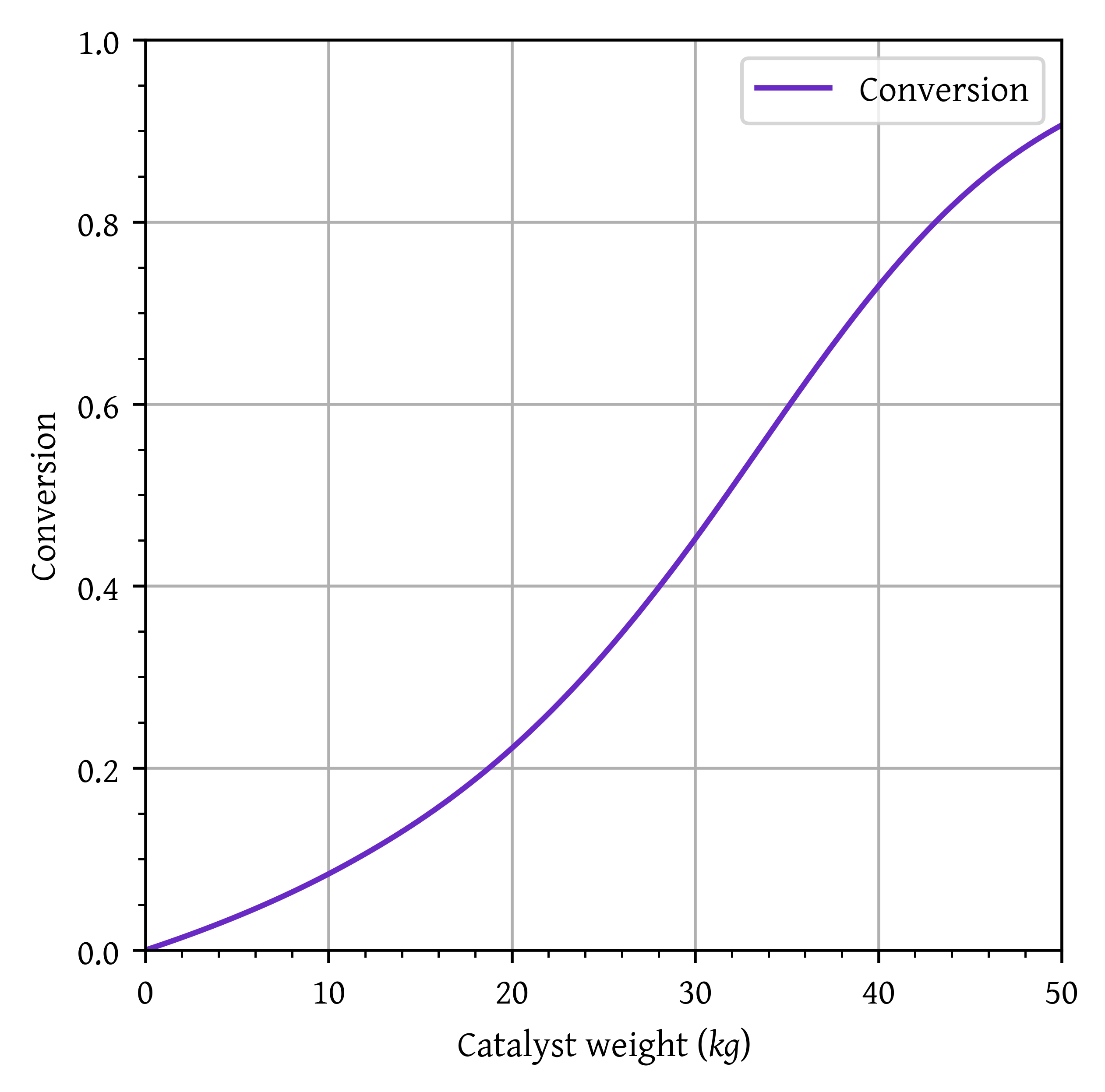
plt.plot(w,T, label='Temperature')

plt.xlim(0,50)


head_margin = (np.max(T) - np.min(T)) * 0.05
ylim_lower = np.min(T)
ylim_upper = np.max(T) + head_margin
plt.ylim(ylim_lower, ylim_upper)

plt.grid()
plt.legend()

plt.xlabel('Catalyst weight ($kg$)')
plt.ylabel('Temperature (K)')

plt.show()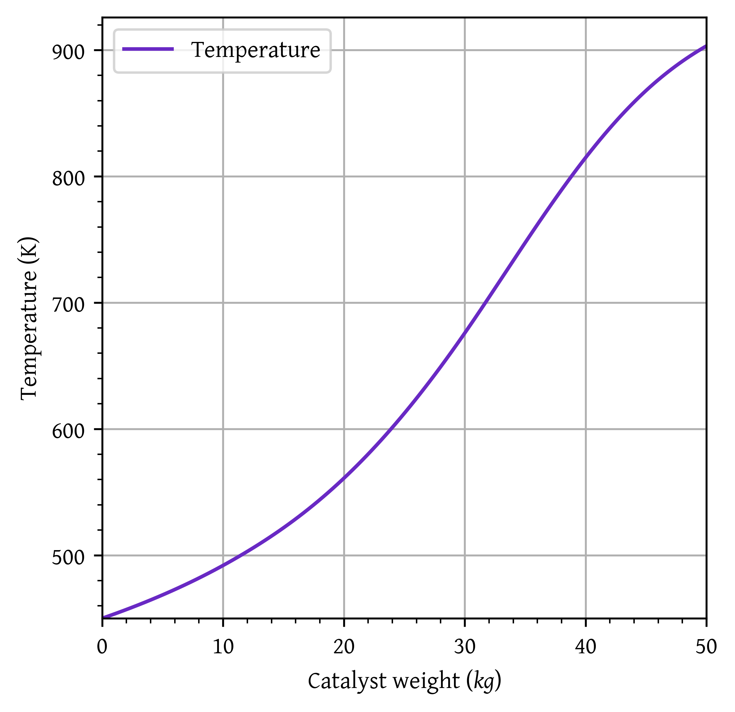
Effect of temperature
T0_range = np.arange(400, 501, 1)
X_final = np.zeros(len(T0_range))
T_final =  np.zeros(len(T0_range))
W_p8 =  np.zeros(len(T0_range))

for i in range(len(T0_range)):

  T0 = T0_range[i]
  args = (ca0, fa0, T0, epsilon, delta_hr_tr, delta_cp, theta)

  # initial condition
  initial_conditions = np.array([0])
  w_final = 50 # kg

  sol = solve_ivp(pfr,
                  [0, w_final],
                 initial_conditions,
                 args=args,
                 dense_output=True)

  w = np.linspace(0,w_final, 1000)
  x = sol.sol(w)[0]
  T  = T0 + x * (-delta_hr_tr)/( np.sum(theta * CP) + x * delta_cp)

  # add values to array for reporting
  X_final[i] = x[-1]
  T_final[i] = T[-1]

  # see if you reach 80% conversion
  if x[-1] > 0.8:
    W_p8[i] = w[x>0.8][0]
plt.plot(T0_range,X_final, label='Conversion')
plt.xlim(T0_range[0],T0_range[-1])
plt.ylim(0,1)
plt.grid()
plt.legend()
plt.xlabel('Inlet temperature (K)')
plt.ylabel('Conversion')
plt.show()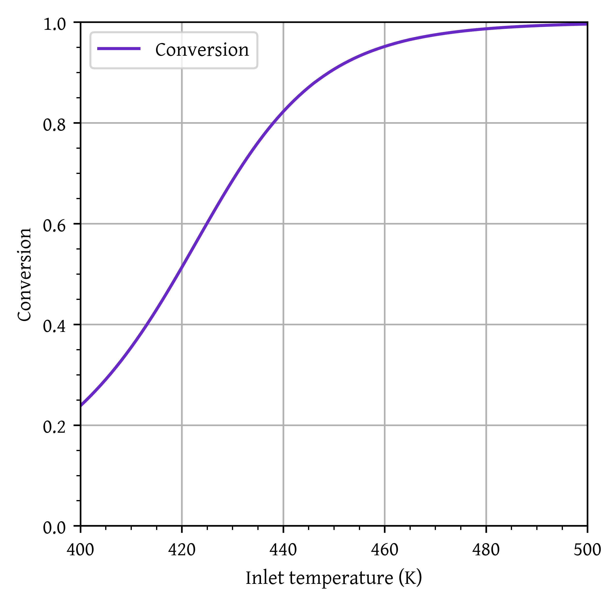
plt.plot(T0_range,T_final, label='Outlet temperature')

plt.xlim(T0_range[0],T0_range[-1])

head_margin = (np.max(T_final) - np.min(T_final)) * 0.05
ylim_lower = np.min(T_final) - head_margin
ylim_upper = np.max(T_final) + head_margin
print (np.max(T_final) + head_margin)
plt.ylim(ylim_lower, ylim_upper)

plt.grid()
plt.legend()

plt.xlabel('Inlet temperature (K)')
plt.ylabel('Temperature (K)')

plt.show()
1022.0467173119888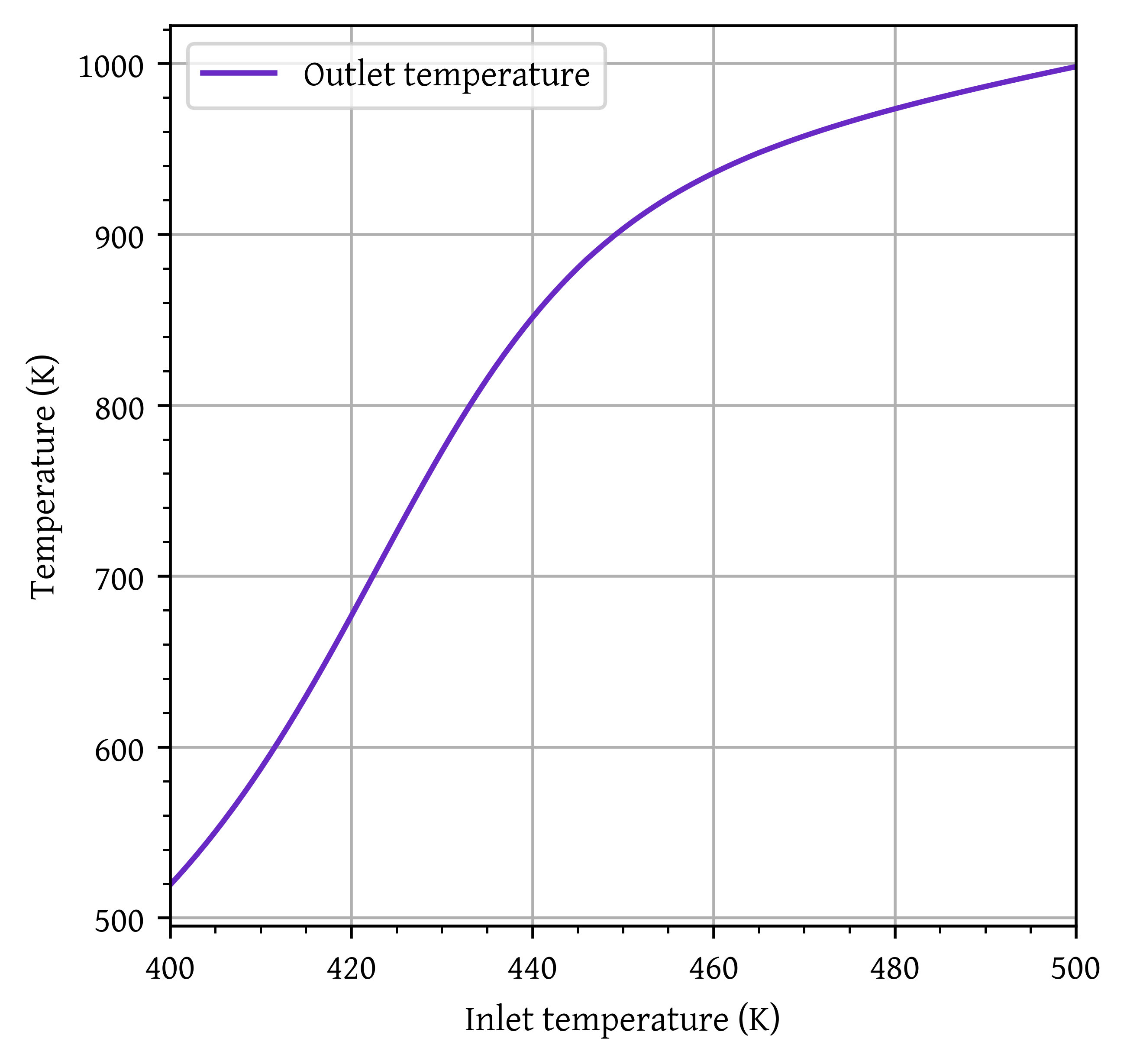
plt.plot(T0_range[W_p8 > 0], W_p8[W_p8 > 0], label='Catalyst weight (kg)')

plt.xlim(T0_range[0],T0_range[-1])
plt.ylim(np.min(W_p8), np.max(W_p8))
plt.legend()

plt.xlabel('Inlet temperature (K)')
plt.ylabel('Catalyst weight (kg)')

plt.fill_between(T0_range, 0, 1,
                 where=W_p8==0,
                 color='gray',
                 alpha=0.3,
                 transform=plt.gca().get_xaxis_transform())

x_pos = np.min(T0_range) + 0.5 * (T0_range[W_p8 > 0][0] - np.min(T0_range))
y_pos = np.min(W_p8) + 0.5 * (np.max(W_p8) - np.min(W_p8))
plt.text(x_pos, y_pos,
         'Conversion < 0.8',
         horizontalalignment='center',
         verticalalignment='center',
         color='black',
         fontsize=10)

plt.show()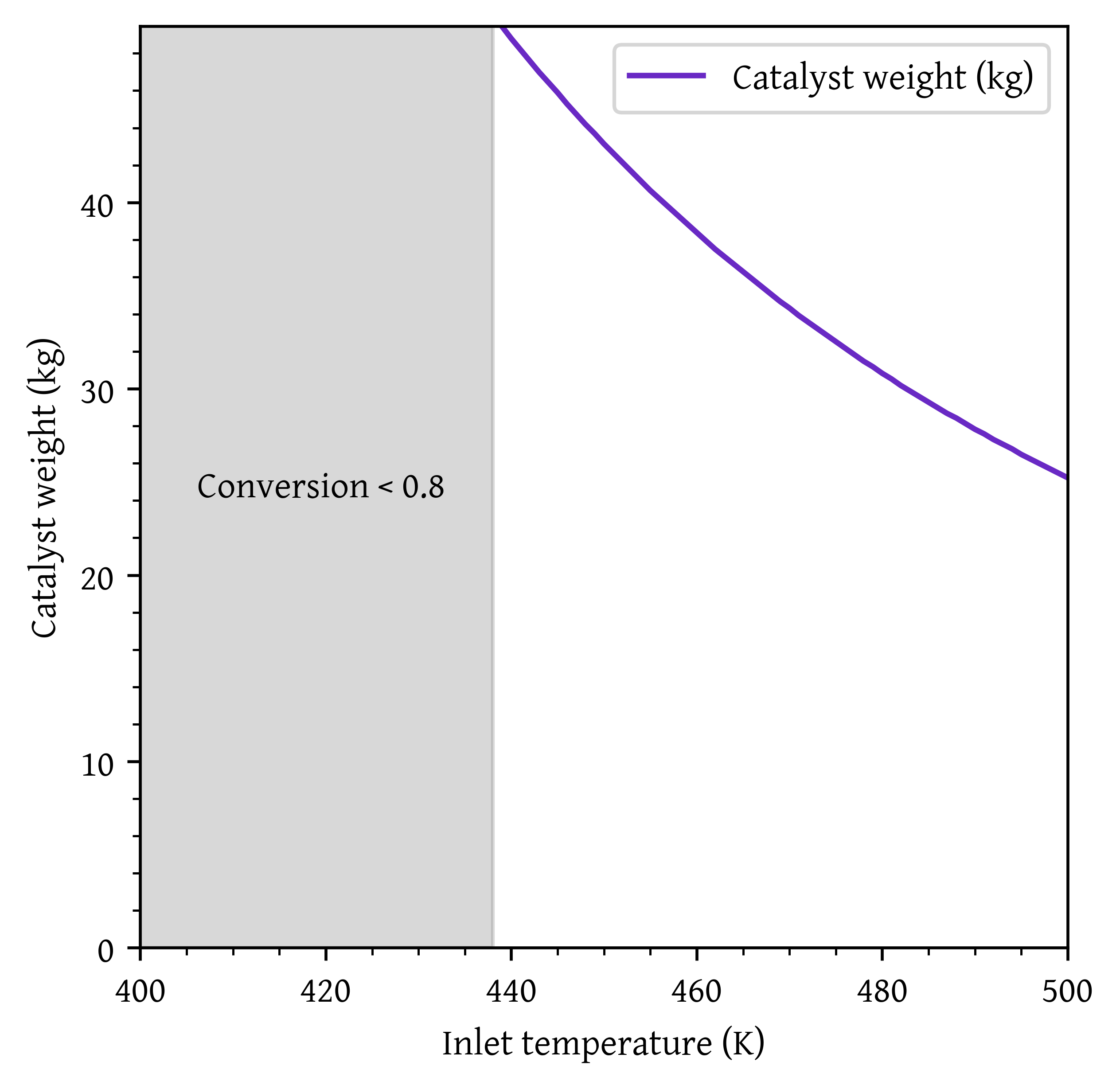
Minimum inlet temperature required to achieve 80% conversion: 439 K
Heat that must be removed along the reactor to maintain isothermal operation:
T0 = 450
args = (ca0, fa0, T0, epsilon, delta_hr_tr, delta_cp, theta)

# initial condition
initial_conditions = np.array([0])
w_final = 50 # kg

sol = solve_ivp(pfr,
                [0, w_final],
                initial_conditions,
                args=args,
                dense_output=True)

w = np.linspace(0,w_final, 1000)
x = sol.sol(w)[0]
T  = T0 + x * (-delta_hr_tr)/( np.sum(theta * CP) + x * delta_cp)
delta_h = delta_hr_tr + delta_cp * (T - TR)
ca = ca0 * (( 1 - x ) / ( 1 + epsilon * x )) * (T0/T)
rate = k(T) * ca # -r_A
heat_removed = -rate*delta_h
plt.plot(w, heat_removed, label='Heat removed')
plt.xlim(np.min(w), np.max(w))
head_margin = (np.max(heat_removed) - np.min(heat_removed)) * 0.05
ylim_upper = np.max(heat_removed) + head_margin
plt.ylim(np.min(heat_removed), ylim_upper)
plt.legend()
plt.xlabel('Catalyst weight (kg)')
plt.ylabel('Heat removed (J/s)')
plt.show()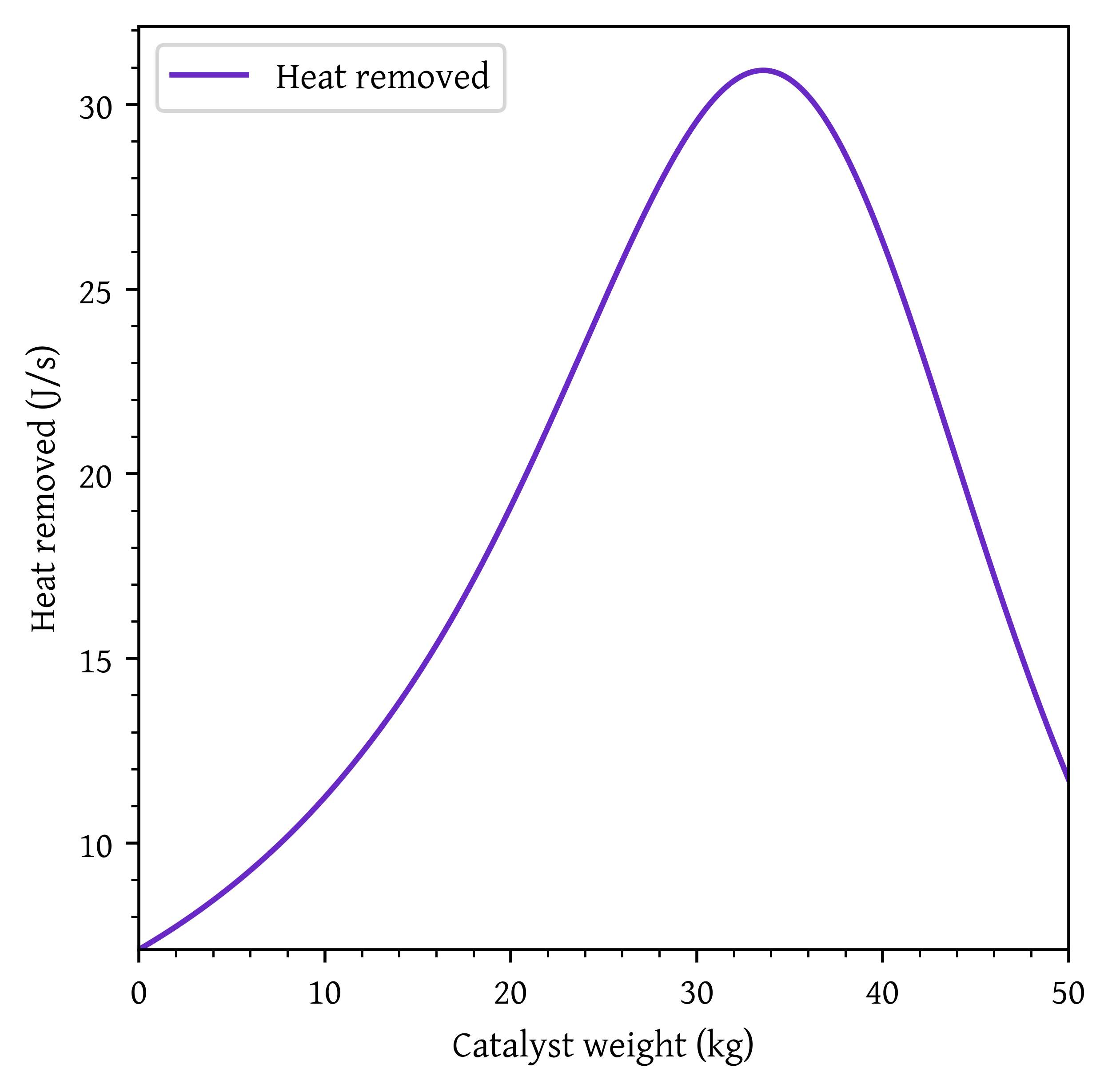
Pressure drop:
def pfr_with_pressure_drop (w, x, *args):
  X,p = x
  (ca0, fa0, T0, epsilon, delta_hr_tr, delta_cp, theta, alpha) = args

  # Calculate T using energy balance
  T  = T0 + X * (-delta_hr_tr)/( np.sum(theta * CP) + X * delta_cp)
  ca = ca0 * p * (( 1 - X )  / ( 1 + epsilon * X )) * (T0/T)

  rate = k(T) * ca # -r_A
  dxdw = rate/fa0
  dpdw = -(alpha/2*p) * (T/T0) * (1 + epsilon * X)

  return [dxdw, dpdw]
T0 = 450
# initial condition
initial_conditions = np.array([0.0, 1.0])
w_final = 50 # kg
alpha1 = 0.0075 # 1/kg
args = (ca0, fa0, T0, epsilon, delta_hr_tr, delta_cp, theta, alpha1)
sol1 = solve_ivp(pfr_with_pressure_drop,
[0, w_final],
initial_conditions,
args=args,
dense_output=True)
w = np.linspace(0,w_final, 1000)
x1 = sol1.sol(w)[0]
T1 = T0 + x1 * (-delta_hr_tr)/( np.sum(theta * CP) + x1 * delta_cp)
p1 = sol1.sol(w)[1]
alpha2 = 0.019 # 1/kg
args = (ca0, fa0, T0, epsilon, delta_hr_tr, delta_cp, theta, alpha2)
sol2 = solve_ivp(pfr_with_pressure_drop,
[0, w_final],
initial_conditions,
args=args,
dense_output=True)
w = np.linspace(0,w_final, 1000)
x2 = sol2.sol(w)[0]
T2 = T0 + x2 * (-delta_hr_tr)/( np.sum(theta * CP) + x2 * delta_cp)
p2 = sol2.sol(w)[1]plt.plot(w,x1, label=f'$\\alpha$ = {alpha1}')
plt.plot(w,x2, label=f'$\\alpha$ = {alpha2}')
plt.xlim(0,50)
plt.ylim(0,1)
plt.grid()
plt.legend()
plt.xlabel('Catalyst weight ($kg$)')
plt.ylabel('Conversion')
plt.show()
plt.plot(w,T1, label=f'$\\alpha$ = {alpha1}')
plt.plot(w,T2, label=f'$\\alpha$ = {alpha2}')

plt.xlim(0,50)

min_t = np.min(np.concatenate((T1, T2)))
max_t = np.max(np.concatenate((T1, T2)))

head_margin = (max_t - min_t) * 0.05
ylim_lower = min_t + head_margin
ylim_upper = max_t + head_margin
plt.ylim(ylim_lower, ylim_upper)

plt.grid()
plt.legend()

plt.xlabel('Catalyst weight ($kg$)')
plt.ylabel('Temperature (K)')

plt.show()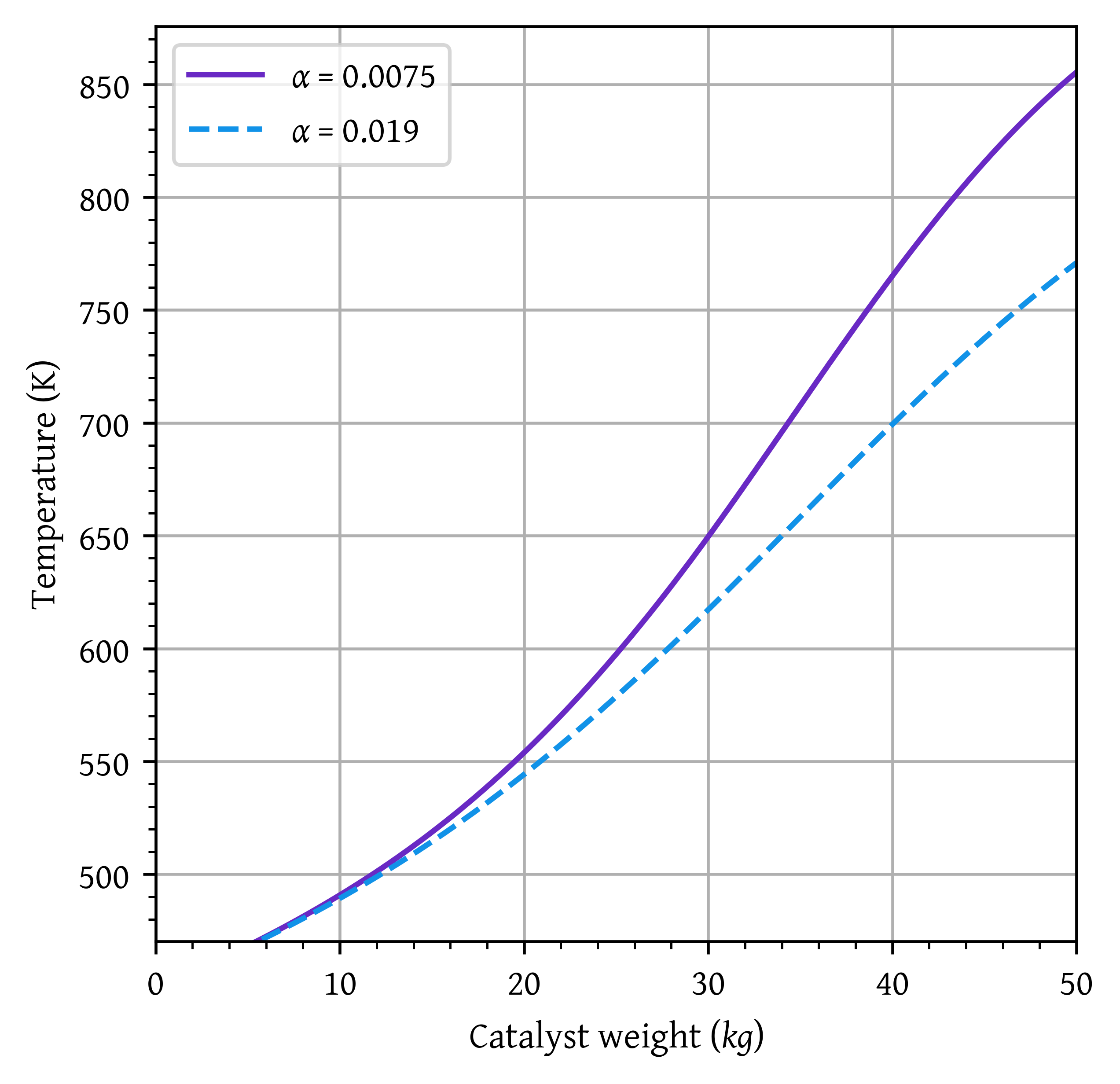
plt.plot(w,p1, label=f'$\\alpha$ = {alpha1}')
plt.plot(w,p2, label=f'$\\alpha$ = {alpha2}')

plt.xlim(0,50)
plt.ylim(0,1)
plt.grid()
plt.legend()

plt.xlabel('Catalyst weight ($kg$)')
plt.ylabel('p $\\left( \\frac{P}{P_0} \\right)$')

plt.show()
P 11-6
The irreversible endothermic vapor-phase reaction follows an elementary rate law
\ce{ CHECOCH3 -> CH2CO + CH4 }
\ce{ A -> B + C }
and is carried out adiabatically in a 500-dm3 PFR. Species A is fed to the reactor at a rate of 10 mol/min and a pressure of 2 atm. An inert stream is also fed to the reactor at 2 atm, as shown in Figure P11-6 B . The entrance temperature of both streams is 1100 K.
Additional information:
k = \exp (34.34 - 34222/T) dm^3/mol \cdot min (T in degrees Kelvin); C_{P_l} = 200 J/ mol \cdot K
C_{P_A} = 170 J/ mol \cdot K; C_{P_B} = 90 J/ mol \cdot K; C_{P_C} = 80 J/ mol \cdot K; \Delta H_{Rx}^\circ = 80000 J/ mol
First derive an expression for C_{A01} as a function of C_{A0} and \Phi_I.
Sketch the conversion and temperature profiles for the case when no inerts are present. Using a dashed line, sketch the profiles when a moderate amount of inerts are added. Using a dotted line, sketch the profiles when a large amount of inerts are added. Qualitative sketches are fine. Describe the similarities and differences between the curves.
Sketch or plot and then analyze the exit conversion as a function of \Phi_I. Is there a ratio of the entering molar flow rates of inerts (I) to A (i.e., \Phi_I = F_{I0}/ F_{A0} at which the conversion is at a maximum? Explain why there “is” or “is not” a maximum.
What would change in parts (b) and (c) if reactions were exothermic and reversible with \Delta H_{Rx}^{\circ} = -80 kJ/mol and K_C = 2 dm^3/mol at 1100 K?
Sketch or plot FB for parts (c) and (d), and describe what you find.
Plot the heat that must be removed along the reactor ( Q vs. V) to maintain isothermal operation for pure A fed and an exothermic reaction.
Solution
import numpy as np
import matplotlib.pyplot as plt
from scipy.integrate import solve_ivp
from scipy.optimize import minimize

k116 = lambda t: np.exp(34.34 - 34222/t)
def pfr116 (V, x, *args):
  X = x[0]
  (ca0, fa0, T0, epsilon, delta_hr_tr, sumCp) = args

  # Calculate T using energy balance
  T = (- delta_hr_tr * X + sumCp* T0)/(sumCp)
  ca = ca0 * (( 1 - X ) / ( 1 + epsilon * X )) * (T0/T)

  rate = k116(T) * ca # -r_A
  dxdw = rate/fa0

  return [dxdw]

# data

R = 0.082 # dm^3 atm / mol K
# A -> B + C
cpA = 170 #J/mol K
cpB = 90 #J/mol K
cpC = 80 #J/mol K
cpI = 200 #J/mol K
delta_hr_tr = 80000 # J/mol

volume = 500 # dm^3
fa0 = 10 # mol/min
P0 = 2 # atm
T0 = 1100 # K

results = {}
thetaIs = [0, 10, 100]

for thetaI in thetaIs:
  fi0 = fa0 * thetaI # mol/min
  ft = fa0 + fi0

  ca0 = P0/(R * T0)
  ci0 = P0/(R * T0)

  ca01 = (ca0 + ci0)/(thetaI + 1)
  epsilon = 1/(1 + thetaI)

  sumCp = cpA + cpI * thetaI

  args = (ca01, fa0, T0, epsilon, delta_hr_tr, sumCp)
  initial_conditions = np.array([0.0])

  sol116 = solve_ivp(pfr116,
                 [0, volume],
                 initial_conditions,
                 args=args,
                 dense_output=True)

  v = np.linspace(0,volume, 1000)
  x = sol116.sol(v)[0]
  T = (- delta_hr_tr * x + sumCp* T0)/(sumCp)

  results[thetaI] = {'v': v, 'x': x, 'T': T}
for thetaI, data in results.items():
plt.plot(data['v'],
data['x'],
label=f'$\\Theta_I$ = {thetaI}')
plt.xlim(0,volume)
plt.ylim(0,1)
plt.grid()
plt.legend()
plt.xlabel('Volume ($dm^3$)')
plt.ylabel('Conversion, $X$')
plt.show()
min_t = []
max_t = []

for thetaI, data in results.items():
  v = data['v']
  T = data['T']
  plt.plot(v, T,
           label=f'$\\Theta_I$ = {thetaI}')

  m = np.min(T)
  min_t.append(m)

  m = np.max(T)
  max_t.append(m)

plt.xlim(0,volume)

min_temp = np.min(min_t)
max_temp = np.max(max_t)
head_margin = (max_temp - min_temp) * 0.05
ylim_lower = min_temp + head_margin
ylim_upper = max_temp + head_margin

plt.ylim(ylim_lower,ylim_upper)

plt.grid()
plt.legend()

plt.xlabel('Volume ($dm^3$)')
plt.ylabel('Temperature (K)')

plt.show()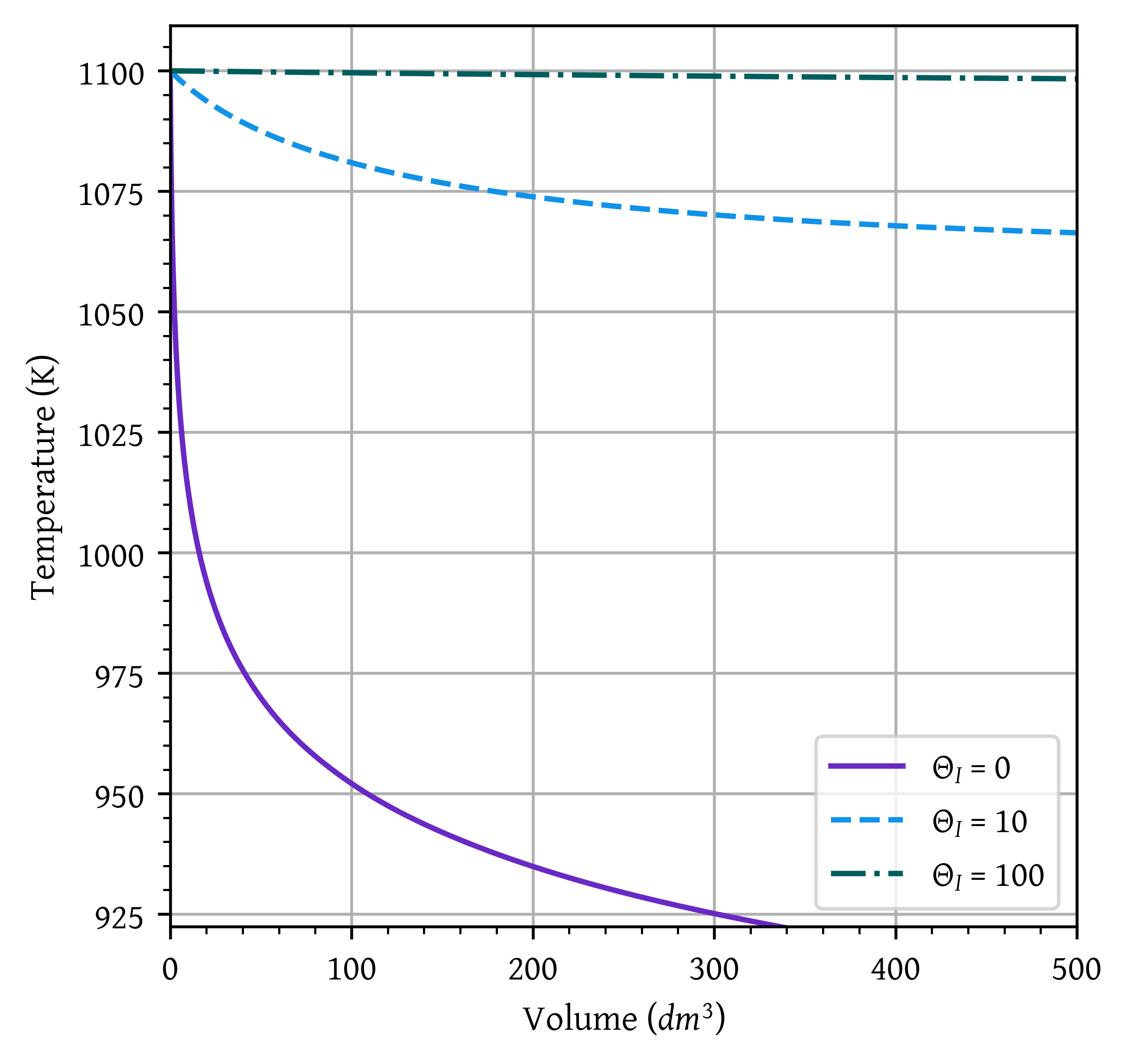
Optimal \Theta_I:
thetaIs = np.arange(0,15 + 0.5,0.5)
conv = []
for thetaI in thetaIs:
  fi0 = fa0 * thetaI # mol/min
  ft = fa0 + fi0

  ca0 = P0/(R * T0)
  ci0 = P0/(R * T0)

  ca01 = (ca0 + ci0)/(thetaI + 1)
  epsilon = 1/(1 + thetaI)

  sumCp = cpA + cpI * thetaI

  args = (ca01, fa0, T0, epsilon, delta_hr_tr, sumCp)
  initial_conditions = np.array([0.0])

  sol116 = solve_ivp(pfr116,
                 [0, volume],
                 initial_conditions,
                 args=args,
                 dense_output=True)

  v = np.linspace(0,volume, 1000)
  x = sol116.sol(v)[0]
  T = (- delta_hr_tr * x + sumCp* T0)/(sumCp)

  conv.append(x[-1])

plt.plot(thetaIs,conv)

plt.xlim(np.min(thetaIs), np.max(thetaIs))

min_x = np.min(conv)
max_x = np.max(conv)
head_margin = (max_x - min_x) * 0.05
ylim_lower = min_x + head_margin
ylim_upper = max_x + head_margin

plt.grid()

plt.xlabel('$\\Theta_I$')
plt.ylabel('Conversion, $X$')

plt.show()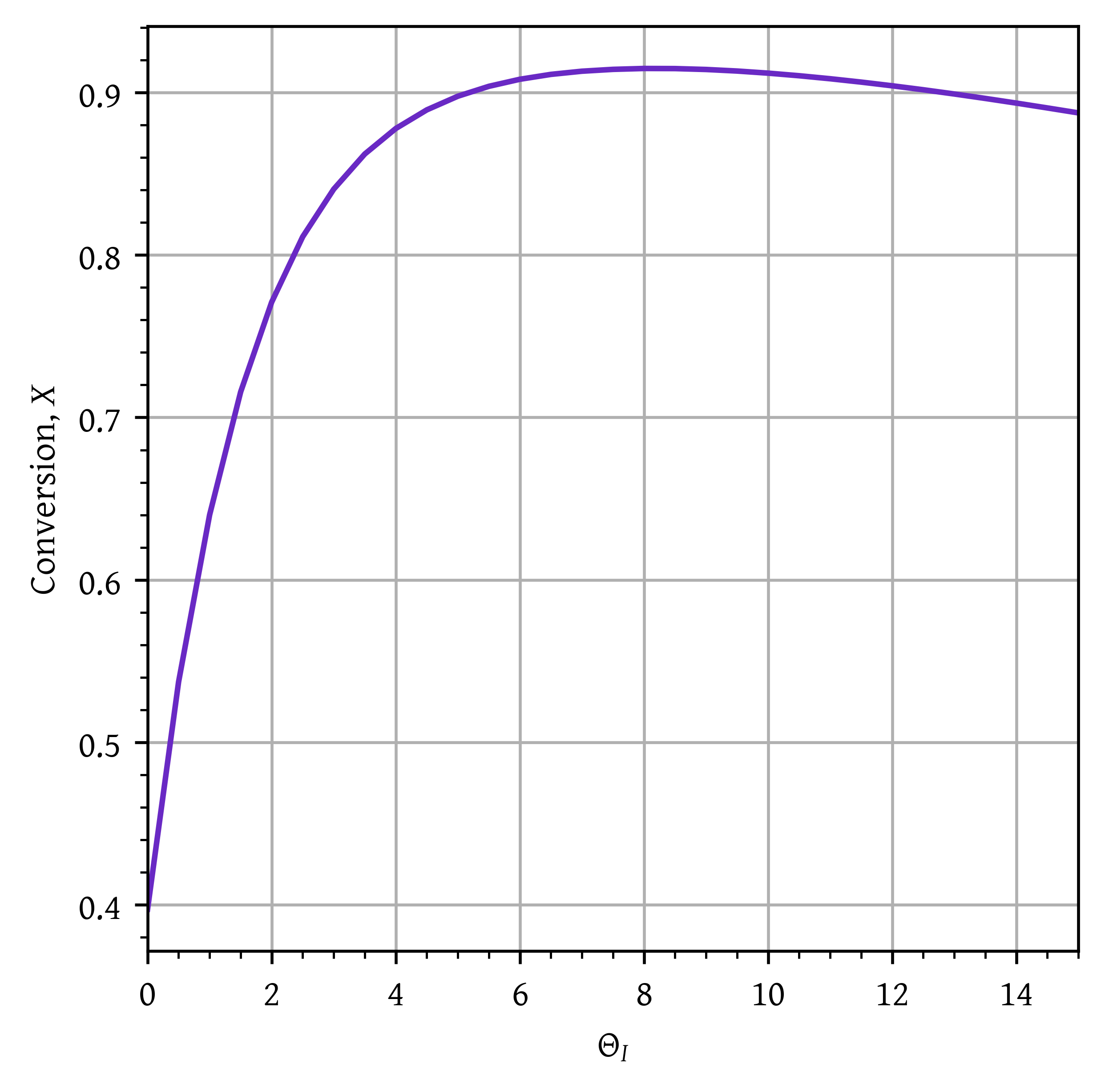
def objective(thetaI):
    ca0 = P0 / (R * T0)
    ci0 = P0 / (R * T0)
    ca01 = (ca0 + ci0) / (thetaI + 1)
    epsilon = 1 / (1 + thetaI)
    sumCp = cpA + cpI * thetaI
    args = (ca01, fa0, T0, epsilon, delta_hr_tr, sumCp)
    initial_conditions = np.array([0.0])

    sol = solve_ivp(pfr116, [0, volume], initial_conditions, args=args, dense_output=True)
    final_x = sol.y[0, -1]  # Get the final conversion
    return -final_x  # Minimize the negative of the final conversion to maximize it

# Constants
R = 0.082  # dm^3 atm / mol K
cpA = 170  # J/mol K
cpI = 200  # J/mol K
delta_hr_tr = 80000  # J/mol
volume = 500  # dm^3
fa0 = 10  # mol/min
P0 = 2  # atm
T0 = 1100  # K

# Optimization setup
thetaI_bounds = (0, 100)  # Define bounds for thetaI as a tuple (min, max)
result = minimize(objective, x0=[10], bounds=[thetaI_bounds], method='L-BFGS-B')

# Display results
optimal_thetaI = result.x[0]
The optimal \Theta_I is 8.187. Maximum conversion = 0.915
P 12-6
The endothermic liquid-phase elementary reaction
\ce { A + B -> 2 C }
proceeds, substantially, to completion in a single steam-jacketed, continuous-stirred reactor (Table P12-6 B ). From the following data, calculate the steady-state reactor temperature:
Reactor volume: 125 gal;
Steam jacket area: 10 ft2
Jacket steam: 150 psig (365.9 ^{\circ}F saturation temperature)
Overall heat-transfer coefficient of jacket, U: 150 Btu/h \cdot ft^2 \cdot ^{\circ}F
Agitator shaft horsepower: 25 hp
Heat of reaction, \Delta H_{Rx}^{\circ} = + 20000 Btu/lb-mol of A (independent of temperature)
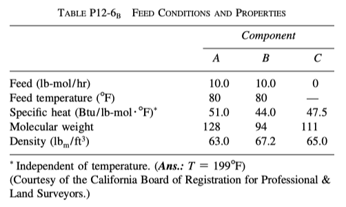
Solution
P 12-21
The irreversible liquid-phase reactions
Reaction 1: \ce{A + B -> 2 C} \;\;\;\; r_{1C} = k_{1C} C_A C_B
Reaction 2: \ce{2 B + C -> D} \;\;\;\; r_{2D} = k_{2D} C_B C_C
are carried out in a PFR with heat exchange. The following temperature profiles were obtained for the reactor and the coolant stream:
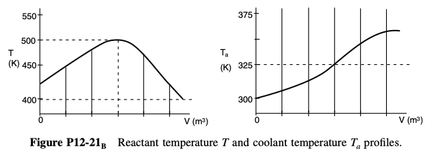
The concentrations of A, B, C, and D were measured at the point down the reactor where the liquid temperature, T, reached a maximum, and they were found to be CA = 0.1, CB = 0.2, CC= 0.5, and CD= 1.5, all in mol/dm3. The product of the overall heat-transfer coefficient and the heat-exchanger area per unit volume, Ua, is 10 cal/s \cdot dm^3 \cdot K. The entering molar flow rate of A is 10 mol/s.
Additional information
C_{P_A}= C_{P_B}=C_{P_C}=30 \, cal/mol/K \;\;\;\; C_{P_D}= 90 \, cal/mol/K, \;\;\;\; C_{P_I}=100 \, cal/mol/K
\Delta H_{Rx1A}^\circ = +5000 \, cal/ molA; \;\;\;\; k_{1C} = 0.043 (dm^3/mol \cdot s) at 400 K
\Delta H_{Rx2B}^\circ = +5000 \, cal/ molB; \;\;\;\; k_{2D} = 0.4 (dm^3/mol \cdot s) \exp 5000 K \left[ \frac{1}{500} - \frac{1}{T}\right]
- What is the activation energy for Reaction (1)?
Solution
Citation
BibTeX citation:
@online{utikar2024,
  author = {Utikar, Ranjeet},
  title = {Solutions to Workshop 07: {Non-isothermal} Reactor Design},
  date = {2024-03-24},
  url = {https://cre.smilelab.dev/content/workshops/07-non-isothermal-reactor-design/solutions.html},
  langid = {en}
}
For attribution, please cite this work as:
Utikar, Ranjeet. 2024. “Solutions to Workshop 07: Non-Isothermal
Reactor Design.” March 24, 2024. https://cre.smilelab.dev/content/workshops/07-non-isothermal-reactor-design/solutions.html.