import numpy as np
from scipy.integrate import solve_ivp
from scipy.optimize import fsolve
import matplotlib.pyplot as plt
from IPython.display import display, Markdown

def batch_reactor(t, y, *args):
  ca, cd, cu = y
  k1, k2, k1A, k2A = args

  r1a = k1 * (ca - cd/k1A)
  r2a = k2 * (ca - cu/k2A)

  dcadt = -r1a -r2a
  dcddt = r1a
  dcudt = r2a

  return [dcadt, dcddt, dcudt]

k1 = 1.0 # 1/min
k2 = 100 # 1/min
k1A = 10.0
k2A = 1.5

ca0 = 1.0

# initial conditions
y0 = [ca0, 0, 0]
args = (k1, k2, k1A, k2A)
t_final = 12

sol = solve_ivp(batch_reactor, [0, t_final], y0, args=args, dense_output=True)

t = np.linspace(0,t_final, 1000)
ca, cd, cu = sol.sol(t)Solutions to workshop 06: Multiple reactions
Lecture notes for chemical reaction engineering
Try following problems from Fogler 5e (Fogler 2016). P 8-3, P 8-4, P 8-7, P 8-9
We will go through some of these problems in the workshop.
P 8-3
The following reactions
\ce{A <=>[ k1 ] D} \qquad -r_{1A} = k_1 \left[ C_A - C_D/K_{1A}\right]
\ce{A <=>[ k2 ] U} \qquad -r_{2A} = k_2 \left[ C_A - C_U/K_{2A}\right]
take place in a batch reactor.
Additional information:
k_1 = 1.0 min–1; K_{1A}= 10
k_2 = 100 min–1; K_{2A} = 1.5
C_{A0} = 1 mol/dm3
Plot and analyze conversion and the concentrations of A, D, and U as a function of time. When would you stop the reaction to maximize the concentration of D? Describe what you find.
When does the maximum concentration of U occur? (Ans.: t = 0.04 min)
What are the equilibrium concentrations of A, D, and U?
What would be the exit concentrations from a CSTR with a space time of 1.0 min? Of 10.0 min? Of 100 min?
Solution
plt.plot(t, ca, label='$C_A$')
plt.plot(t, cd, label='$C_D$')
plt.plot(t, cu, label='$C_U$')

plt.xlabel('time (min)')
plt.ylabel('Concentration ($mol/dm^3$)')

# Setting x and y axis limits
plt.xlim(0, t_final)
plt.ylim(0, ca0)

plt.legend()
plt.show()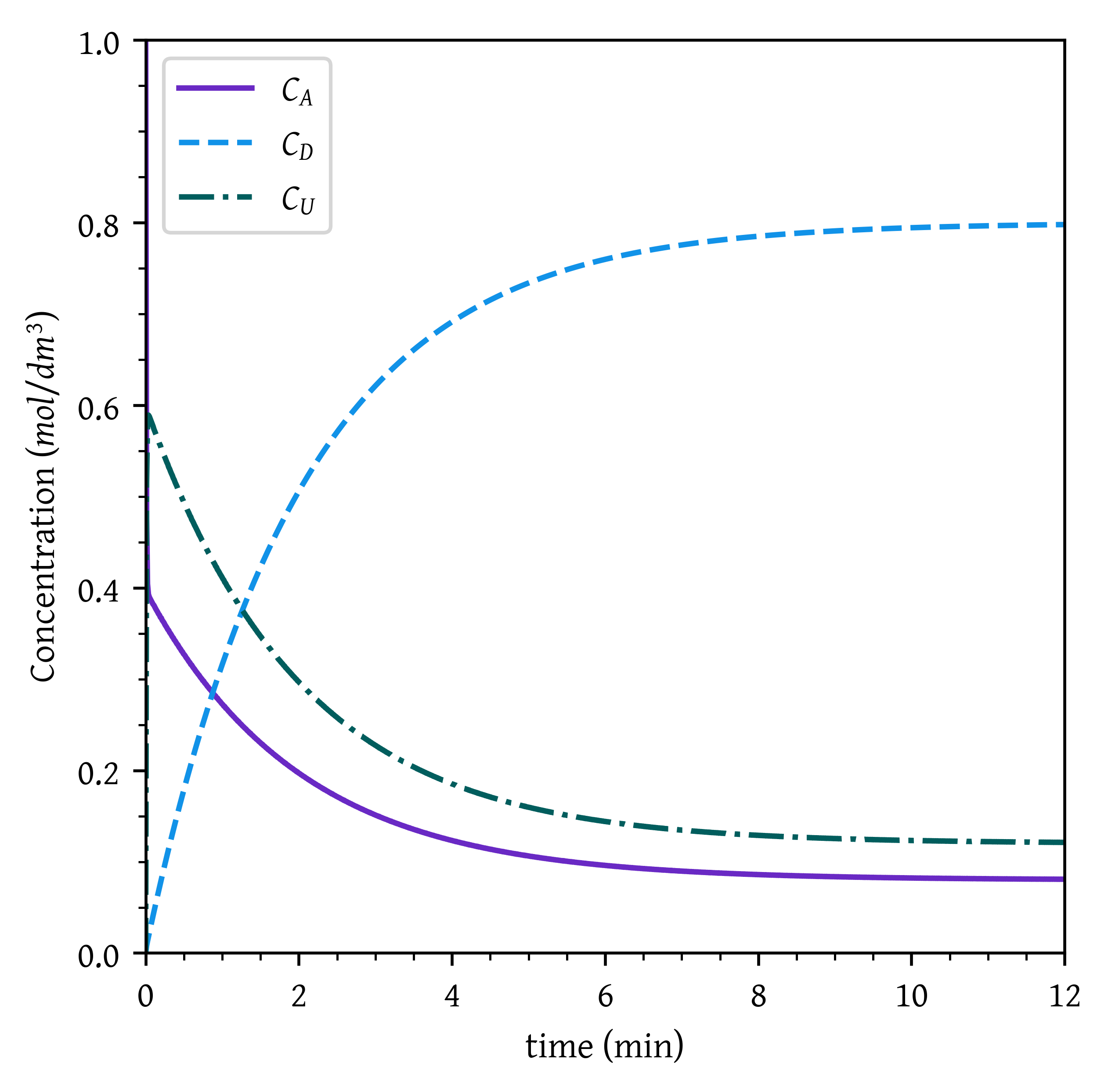
cumax_idx = np.argmax(cu)
tumax = t[cumax_idx]
cumax = cu[cumax_idx]
Maximum concentration of U, C_U = C_{Umax} = 0.59 mol/dm^3 occurs at t_{Umax} = 0.04 min
As C_D keeps on increasing with time until the equilibrium is reached, To maximize C_D, stop the reaction after equilibrium is reached.
cae = ca[-1]
cde = cd[-1]
cue = cu[-1]
Equilibrium concentrations
C_{Ae} = 0.08 mol/dm^3
C_{De} = 0.80 mol/dm^3
C_{Ue} = 0.12 mol/dm^3
def cstr(vars, *args):
  ca, cd, cu = vars
  t, k1, k2, k1A, k2A = args

  r1a = k1 * (ca - cd/k1A)
  r2a = k2 * (ca - cu/k2A)

  eq1 = ca0 - ca - t * (r1a + r2a)
  eq2 = -cd + t * r1a
  eq3 = -cu + t * r2a

  return [eq1, eq2, eq3]


initial_guess = [ca0, 0, 0]
times = [1, 10, 100]

md = ""

for tau in times:
  args = (tau, k1, k2, k1A, k2A)
  ca, cd, cu = fsolve(cstr, initial_guess, args=args)

  md += (
    f"At $\\tau$ = {tau:.2f} min.:\n"
    f"$C_A$ = {ca:.2f} $mol/dm^3$,\n"
    f"$C_D$ = {cd:.2f} $mol/dm^3$,\n"
    f"$C_U$ = {cu:.2f} $mol/dm^3$ \n\n"
  )

display(Markdown(md))
At \tau = 1.00 min.: C_A = 0.30 mol/dm^3, C_D = 0.27 mol/dm^3, C_U = 0.44 mol/dm^3
At \tau = 10.00 min.: C_A = 0.13 mol/dm^3, C_D = 0.67 mol/dm^3, C_U = 0.20 mol/dm^3
At \tau = 100.00 min.: C_A = 0.09 mol/dm^3, C_D = 0.78 mol/dm^3, C_U = 0.13 mol/dm^3
P 8-4
Consider the following system of gas-phase reactions:
\begin{aligned} \ce{A -> X} & \quad r_X = k_1 C_A^{1/2} & \quad k_1 &= 0.004 \ \left(mol/dm^3\right)^{1/2} \cdot min^{-1} \\ \ce{A -> B} & \quad r_B = k_2 C_A & \quad k_2 &= 0.3 \ min^{-1} \\ \ce{A -> Y} & \quad r_Y = k_3 C_A^{2} & \quad k_3 &= 0.25 \ dm^3/mol \cdot min^{-1} \\ \end{aligned}
B is the desired product, and X and Y are foul pollutants that are expensive to get rid of. The specific reaction rates are at 27 ^{\circ}C. The reaction system is to be operated at 27 ^{\circ}C and 4 atm. Pure A enters the system at a volumetric flow rate of 10 dm3/min.
Sketch the instantaneous selectivities (S_{B/X}, S_{B/Y}, \text{and} \, S_{B/XY} = r_B /(r_X + r_Y)) as a function of the concentration of CA.
Consider a series of reactors. What should be the volume of the first reactor?
What are the effluent concentrations of A, B, X, and Y from the first reactor?
What is the conversion of A in the first reactor?
If 99% conversion of A is desired, what reaction scheme and reactor sizes should you use to maximize S_{B/XY}?
Suppose that E1 = 20,000 cal/mol, E2=10,000 cal/mol, and E3=30,000 cal/mol. What temperature would you recommend for a single CSTR with a space time of 10 min and an entering concentration of A of 0.1 mol/dm3 ?
Solution
import numpy as np
from scipy.integrate import solve_ivp
from scipy.optimize import fsolve
from scipy.optimize import minimize_scalar
from scipy.integrate import quad
import matplotlib.pyplot as plt
from IPython.display import display, Markdown


rx = lambda ca: 0.004 * ca**0.5
rb = lambda ca: 0.3 * ca
ry = lambda ca: 0.25 * ca**2

sbx = lambda ca: rb(ca)/rx(ca)
sby = lambda ca: rb(ca)/ry(ca)
sbxy = lambda ca: rb(ca)/(rx(ca) + ry(ca))

ca = np.linspace(1e-4,1,100)
plt.plot(ca,sbx(ca))
plt.xlabel('$C_A$ ($mol/dm^3$)')
plt.ylabel('$S_{B/X}$')
# Setting x and y axis limits
plt.xlim(0, ca[-1])
plt.ylim(0, np.ceil(sbx(ca[-1])))
plt.show()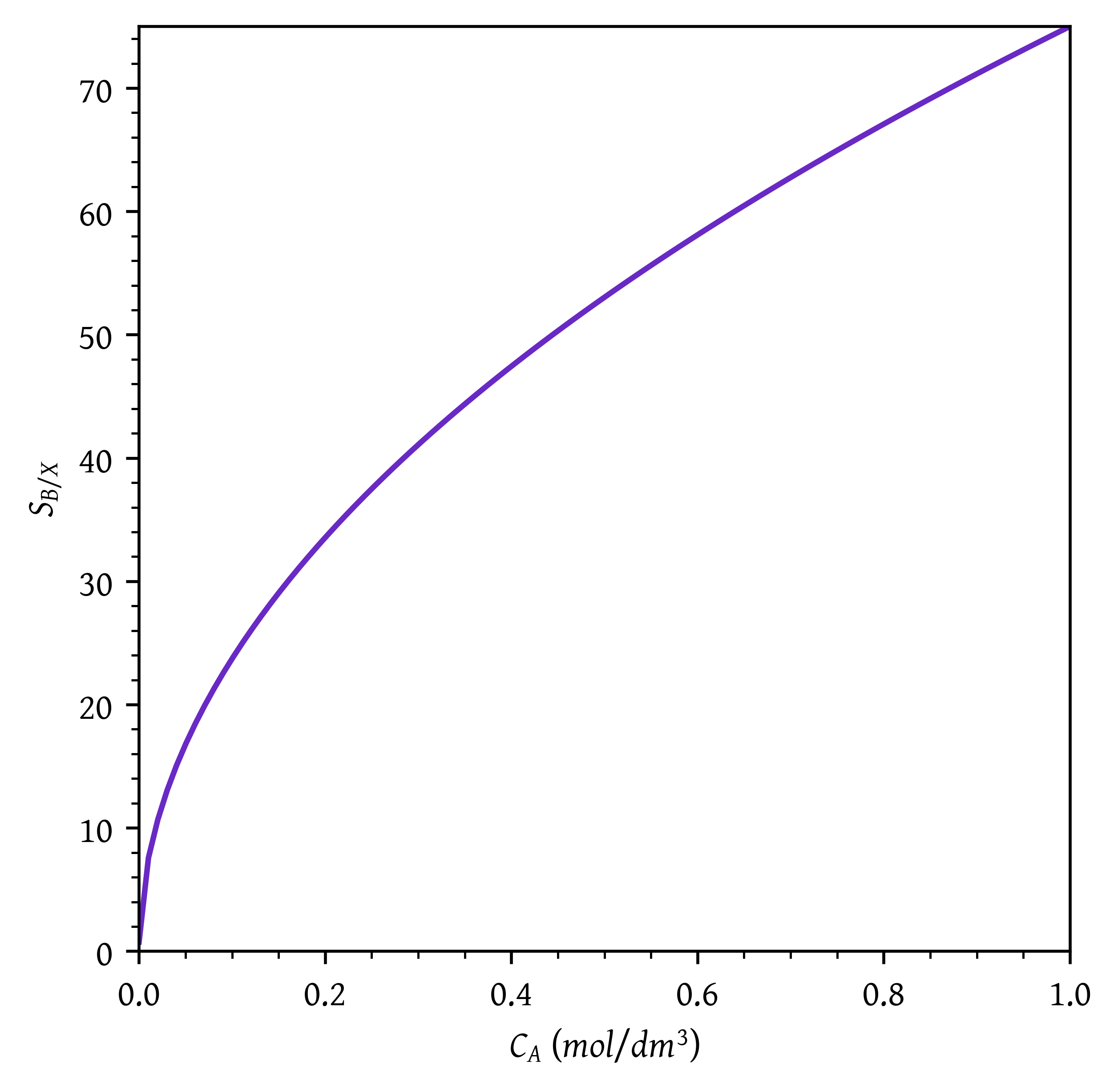
plt.plot(ca,sby(ca))

plt.xlabel('$C_A$ ($mol/dm^3$)')
plt.ylabel('$S_{B/Y}$')

# Setting x and y axis limits
plt.xlim(0, ca[-1])
plt.ylim(0, 20)

plt.show()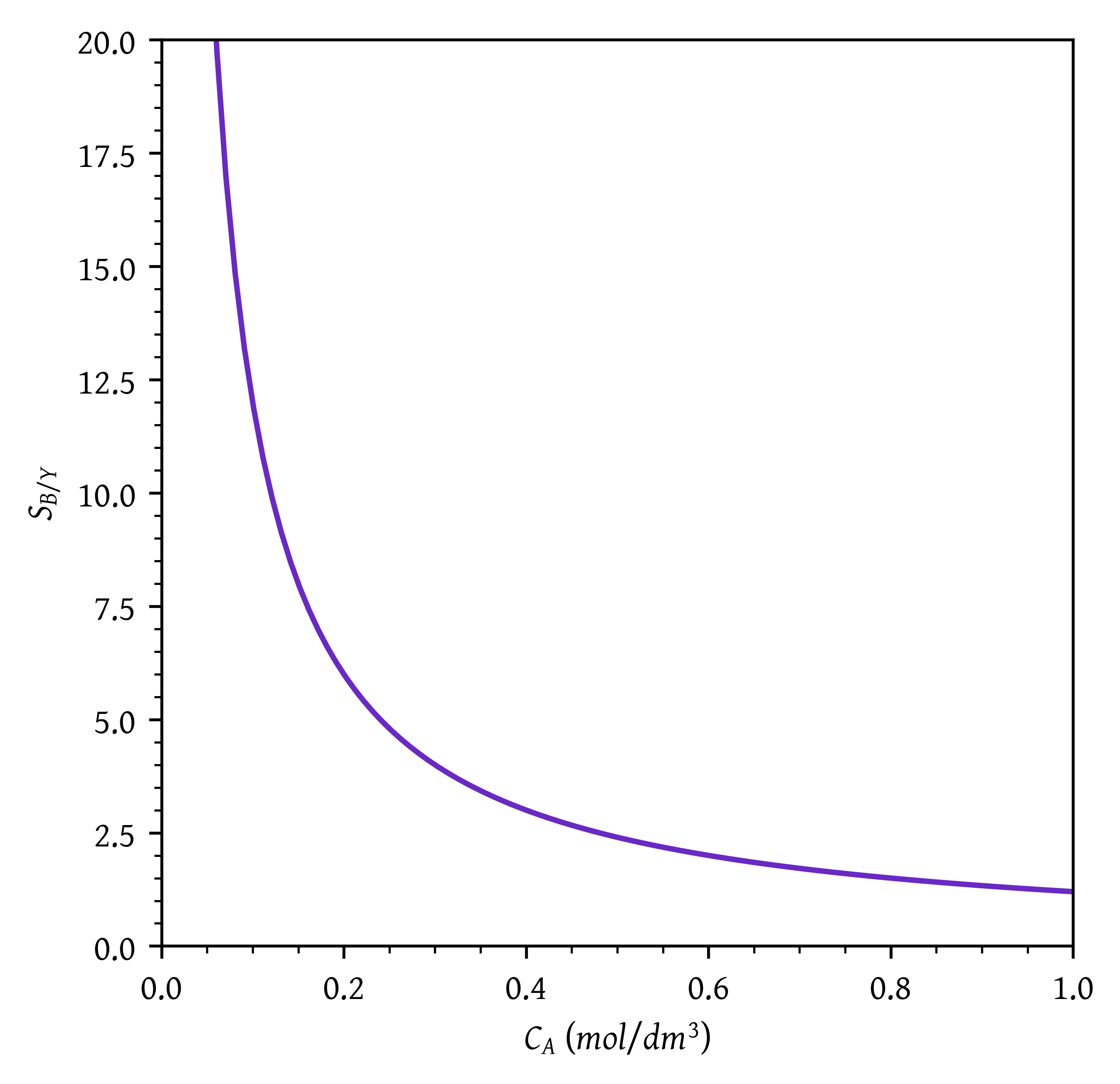
plt.plot(ca,sbxy(ca))

plt.xlabel('$C_A$ ($mol/dm^3$)')
plt.ylabel('$S_{B/XY}$')

# Setting x and y axis limits
plt.xlim(0, ca[-1])
plt.ylim(0, 12)

plt.show()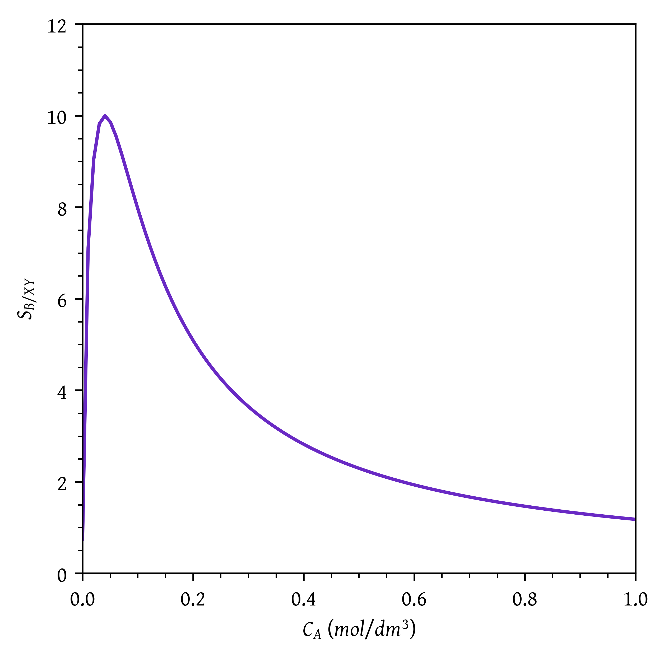
# Maximize S_B/XY
bounds=(1e-4, 1)
# Maximize the selectivity by minimizing the negative of the selectivity function
result = minimize_scalar(lambda ca: -sbxy(ca), method='bounded', bounds=bounds)

camax = result.x
sbxy_max = sbxy(camax)
Maximum concentration of A, C_{Amax} = 0.04 mol/dm^3
Maximum selectivity = 10.00
The CSTR operates at exit concentration of 0.04 mol/dm^3
T = 27 + 273.15 # K
v0 = 10 # dm^3/min
P = 4 # atm
ya0 = 1 # pure A
R = 0.082

ca0 = ya0 * P /(R * T)

rate = rx(camax) + rb(camax) + ry(camax)
v_cstr = v0 * (ca0 - camax)/ rate- C_{A0} = 0.163 mol/dm^3
- V_{CSTR} = 92.81 dm^3
tau_cstr = v_cstr/v0

cb_cstr = tau_cstr* rb(camax)
cx_cstr = tau_cstr* rx(camax)
cy_cstr = tau_cstr* ry(camax)
Exit concentration of CSTR
- C_{B} = 1.114e-01 mol/dm^3
- C_{X} = 7.425e-03 mol/dm^3
- C_{Y} = 3.713e-03 mol/dm^3
x_cstr = (ca0 - camax)/ca0Conversion in first reactor = 0.75
fa0 = ca0*v0
fa0_by_ra = fa0/(rb(ca) + rx(ca) + ry(ca))
x = (ca0 - ca)/ca0
plt.plot(x,fa0_by_ra)

plt.xlabel('$X$')
plt.ylabel('$F_{A0}/-r_A$')

# Setting x and y axis limits
plt.xlim(0, 1)
# plt.ylim(0, 10000)

plt.show()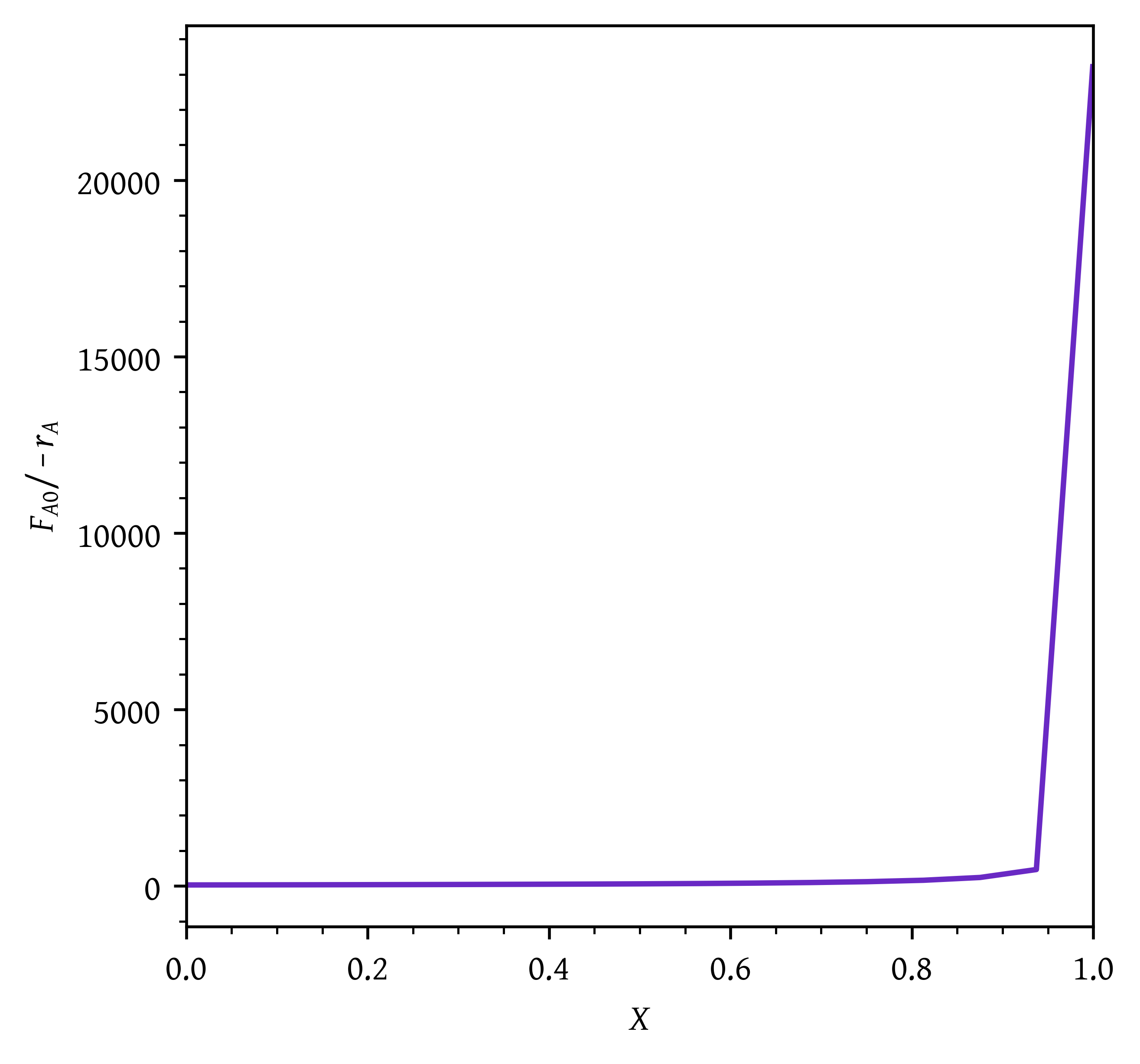
def pfr(x, *args):
  fa0 = args[0]

  ca = ca0 * (1 - x)
  return fa0/(rb(ca) + rx(ca) + ry(ca))

x_start = x_cstr
x_end = 0.99

v_pfr, _ = quad(pfr, x_start, x_end, args=(fa0))PFR volume required to achieve final conversion of 0.99 = 91.18 dm^3
e1 = 20000
e2 = 10000
e3 = 30000

k1 = lambda T: 0.004 * np.exp((e1/1.98) * ((1/T) - (1/300)))
k2 = lambda T: 0.3   * np.exp((e2/1.98) * ((1/T) - (1/300)))
k3 = lambda T: 0.25  * np.exp((e3/1.98) * ((1/T) - (1/300)))

rxt = lambda ca,T: k1(T) * ca**0.5
rbt = lambda ca,T: k2(T) * ca
ryt = lambda ca,T: k3(T) * ca**2

sbxt = lambda ca,T: rbt(ca,T)/rxt(ca,T)
sbyt = lambda ca,T: rbt(ca,T)/ryt(ca,T)
sbxyt = lambda ca,T: rbt(ca,T)/(rxt(ca,T) + ryt(ca,T))

tau = 10
ca0 = 0.1

initial_guess = [ca0, 0, 0, 0]

def cstr_btx(vars, *args):
  ca, cx, cb, cy = vars
  tau, T = args

  r1 = rxt(ca,T)
  r2 = rbt(ca,T)
  r3 = ryt(ca,T)

  eq1 = ca0 - ca - tau * (r1 + r2 + r3)
  eq2 = -cx + tau * r1
  eq3 = -cb + tau * r2
  eq4 = -cy + tau * r3

  return [eq1, eq2, eq3, eq4]

# Function to solve the CSTR equations for a given temperature
def maximize_cb(T):
    args = (tau, T)
    ca, cx, cb, cy = fsolve(cstr_btx, initial_guess, args=args)
    return -cb

result = minimize_scalar(maximize_cb, bounds=(275, 400), method='bounded')

optimal_temp = result.x
max_cb = -result.fun


temps = np.linspace(275,400,100)
cb_values = []

for temp in temps:
  args = (tau, temp)
  ca, cx, cb, cy = fsolve(cstr_btx, initial_guess, args=args)
  cb_values.append(cb)

cb_values = np.array(cb_values)
temps = np.array(temps)

max_cb_index = np.argmax(cb_values)
max_cb_temp = temps[max_cb_index]
max_cb = cb_values[max_cb_index]

plt.plot(temps, cb_values)
plt.scatter([max_cb_temp], [max_cb], zorder=5)

# plt.axvline(x=max_cb_temp, color='gray', linestyle='--', lw=1)
# plt.axhline(y=max_cb, color='gray', linestyle='--', lw=1)

plt.plot([max_cb_temp, max_cb_temp], [0, max_cb], color='gray', linestyle='--', lw=1)  # Vertical line to curve
plt.plot([min(temps), max_cb_temp], [max_cb, max_cb], color='gray', linestyle='--', lw=1)  # Horizontal line to curve

plt.xlabel('Temperature (K)')
plt.ylabel('Concentration of B ($mol/dm^3$)')

# Setting x and y axis limits
plt.xlim(275, 400)
plt.ylim(0, 0.08)

plt.show()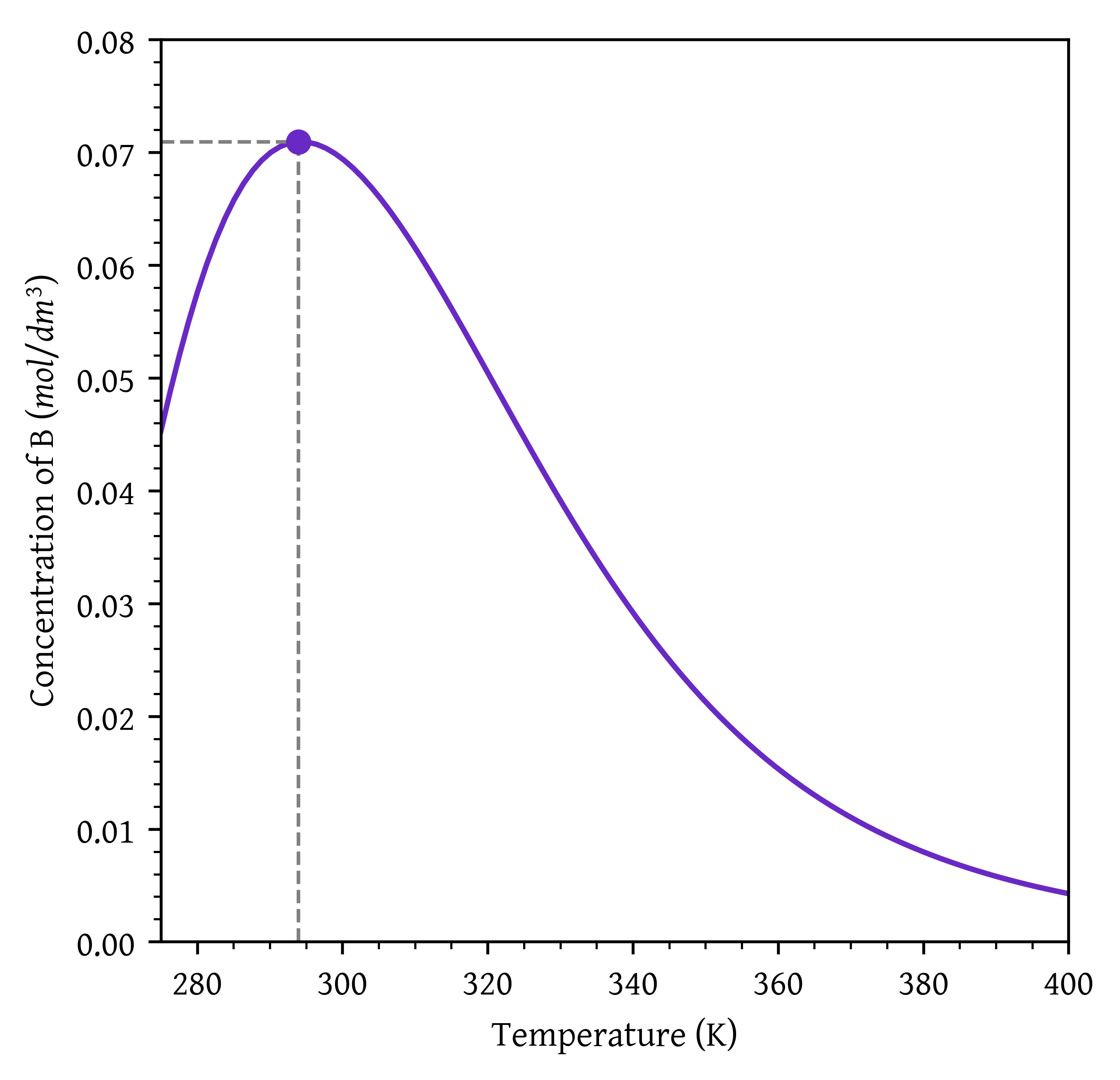
- Optimal temperature for maximizing C_B = 294.26 K. Maximum C_B= 0.07
P 8-9
The elementary liquid-phase series reaction
\ce{A ->[ k1 ] B ->[ k2 ] C}
is carried out in a 500-dm3 batch reactor. The initial concentration of A is 1.6 mol/dm3. The desired product is B, and separation of the undesired product C is very difficult and costly. Because the reaction is carried out at a relatively high temperature, the reaction is easily quenched.
Plot and analyze the concentrations of A, B, and C as a function of time. Assume that each reaction is irreversible, with k_1 = 0.4 \, h^{-1} and k_2 = 0.01 \, h^{-1}.
Plot and analyze the concentrations of A, B, and C as a function of time when the first reaction is reversible, with k_{-1} = 0.3 \, h^{-1}.
Plot and analyze the concentrations of A, B, and C as a function of time for the case where both reactions are reversible, with k_{-2} = 0.005 \, h^{-1}.
Compare (a), (b), and (c) and describe what you find.
Vary k_1, k_2, k_{-1}, \text{and} \, k_{-2}. Explain the consequence of k_1 > 100 and k_2 < 0.1 and with k_{-1} = k_{-2} = 0 and with k_{-2}= 1, k_{-1} = 0, and k_{-2} = 0.25.
Solution
import numpy as np
from scipy.integrate import solve_ivp
import matplotlib.pyplot as plt

def batch_reactor_a(t, y, *args):
  ca, cb, cc = y
  k1, k2 = args

  r1a = k1 * ca
  r2b = k2 * cb

  dcadt = - r1a
  dcbdt = r1a - r2b
  dccdt = r2b

  return [dcadt, dcbdt, dccdt]

k1 = 0.4 # 1/h
k2 = 0.01

ca0 = 1.6

# initial conditions
y0 = [ca0, 0, 0]
args = (k1, k2)
t_final = 50

sol = solve_ivp(batch_reactor_a, [0, t_final], y0, args=args, dense_output=True)

t = np.linspace(0,t_final, 1000)
ca, cb, cc = sol.sol(t)
plt.plot(t, ca, label='$C_A$')
plt.plot(t, cb, label='$C_B$')
plt.plot(t, cc, label='$C_C$')
plt.xlabel('time (h)')
plt.ylabel('Concentration ($mol/dm^3$)')
# Setting x and y axis limits
plt.xlim(0, t_final)
plt.ylim(0, ca0)
plt.legend()
plt.show()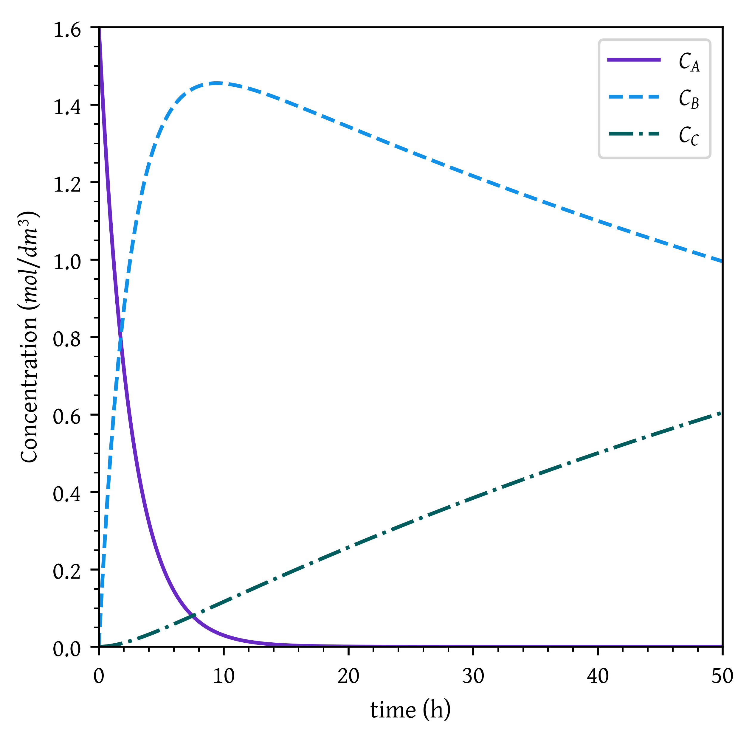
def batch_reactor_b(t, y, *args):
ca, cb, cc = y
k1, k2, km1 = args
r1a = k1 * ca
r1b = km1 * cb
r2b = k2 * cb
dcadt = - r1a + r1b
dcbdt = r1a -r1b - r2b
dccdt = r2b
return [dcadt, dcbdt, dccdt]
km1 = 0.3
# initial conditions
y0 = [ca0, 0, 0]
args = (k1, k2, km1)
t_final = 50
sol = solve_ivp(batch_reactor_b, [0, t_final], y0, args=args, dense_output=True)
t = np.linspace(0,t_final, 1000)
ca, cb, cc = sol.sol(t)plt.plot(t, ca, label='$C_A$')
plt.plot(t, cb, label='$C_B$')
plt.plot(t, cc, label='$C_C$')
plt.xlabel('time (h)')
plt.ylabel('Concentration ($mol/dm^3$)')
# Setting x and y axis limits
plt.xlim(0, t_final)
plt.ylim(0, ca0)
plt.legend()
plt.show()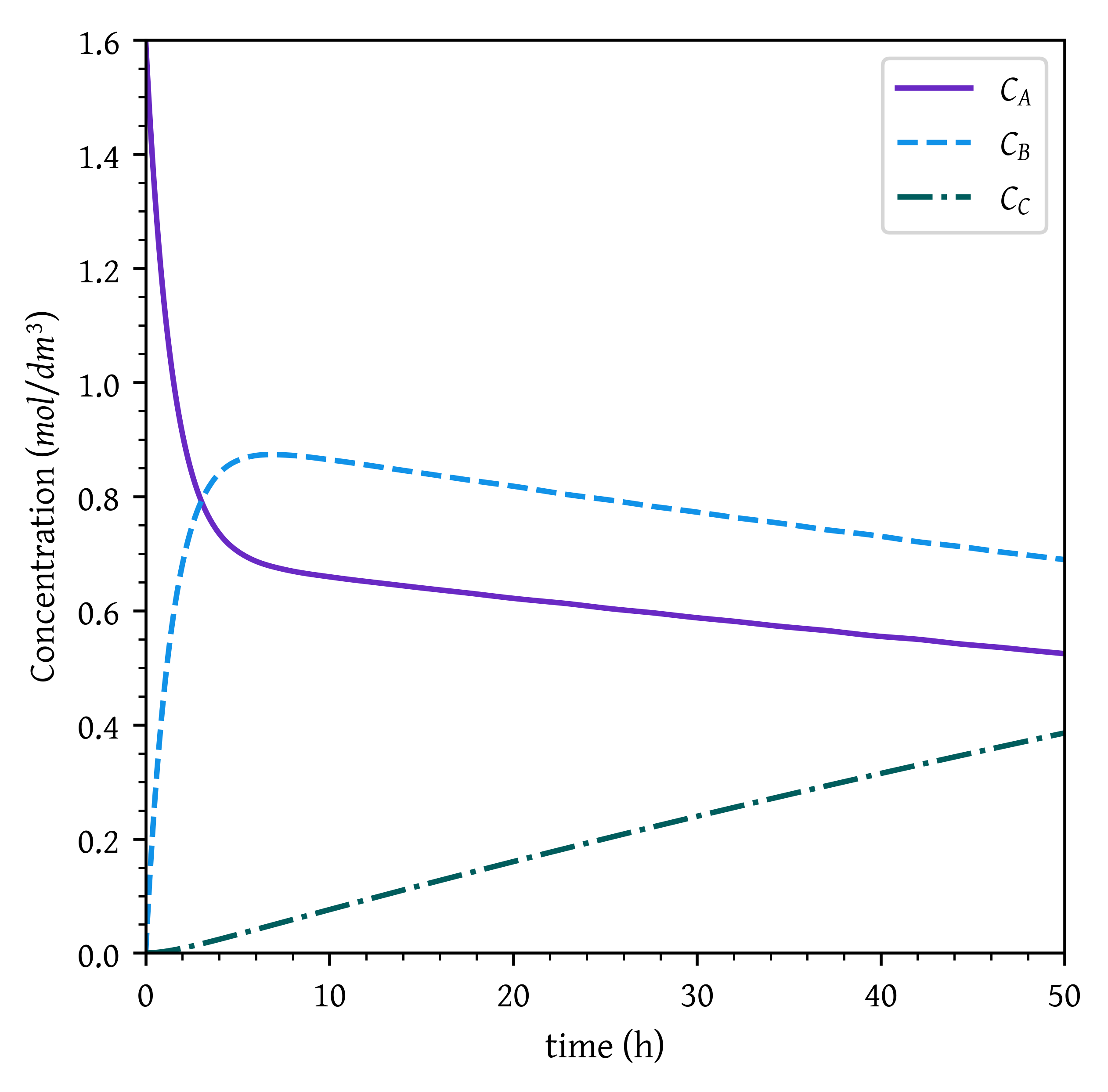
def batch_reactor_c(t, y, *args):
ca, cb, cc = y
k1, k2, km1, km2 = args
r1a = k1 * ca
r1b = km1 * cb
r2b = k2 * cb
r2c = km2 * cc
dcadt = - r1a + r1b
dcbdt = r1a -r1b - r2b + r2c
dccdt = r2b - r2c
return [dcadt, dcbdt, dccdt]
km1 = 0.3
km2 = 0.005
# initial conditions
y0 = [ca0, 0, 0]
args = (k1, k2, km1, km2)
t_final = 50
sol = solve_ivp(batch_reactor_c, [0, t_final], y0, args=args, dense_output=True)
t = np.linspace(0,t_final, 1000)
ca, cb, cc = sol.sol(t)plt.plot(t, ca, label='$C_A$')
plt.plot(t, cb, label='$C_B$')
plt.plot(t, cc, label='$C_C$')
plt.xlabel('time (h)')
plt.ylabel('Concentration ($mol/dm^3$)')
# Setting x and y axis limits
plt.xlim(0, t_final)
plt.ylim(0, ca0)
plt.legend()
plt.show()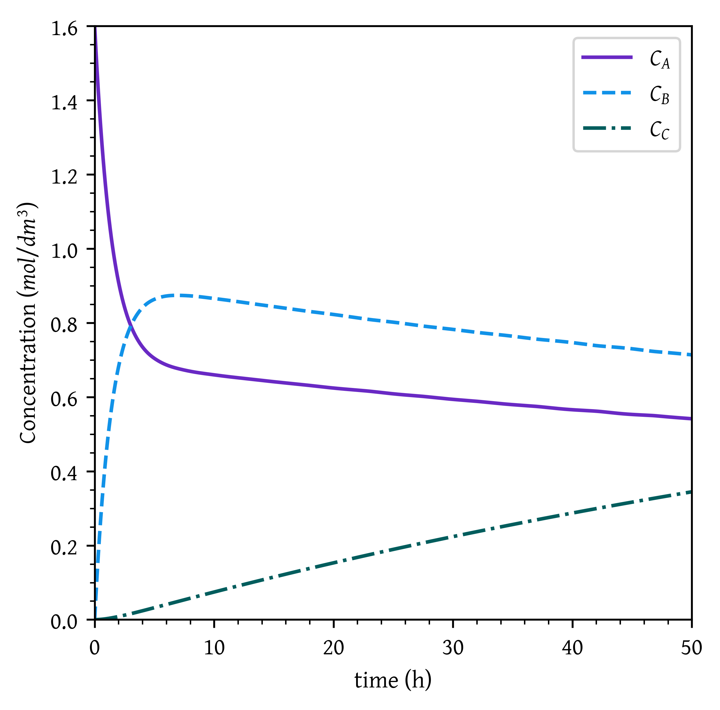
k1 = 100
k2 = 1
km1 = 0
km2 = 0
# initial conditions
y0 = [ca0, 0, 0]
args = (k1, k2, km1, km2)
t_final = 10
sol = solve_ivp(batch_reactor_c, [0, t_final], y0, args=args, dense_output=True)
t = np.linspace(0,t_final, 1000)
ca, cb, cc = sol.sol(t)
plt.plot(t, ca, label='$C_A$')
plt.plot(t, cb, label='$C_B$')
plt.plot(t, cc, label='$C_C$')

plt.xlabel('time (h)')
plt.ylabel('Concentration ($mol/dm^3$)')

# Setting x and y axis limits
plt.xlim(0, t_final)
plt.ylim(0, ca0)

plt.legend()
plt.show()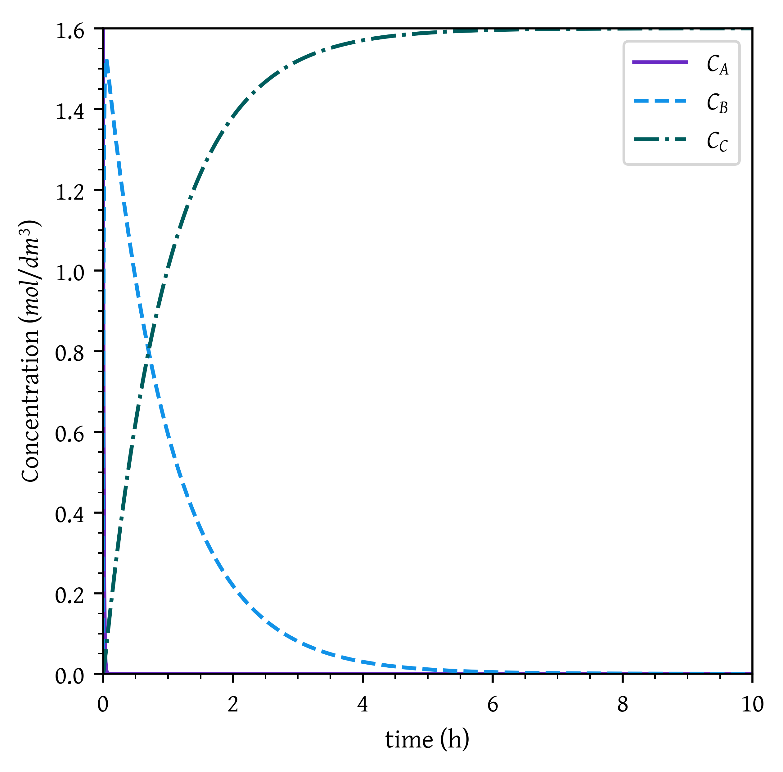
When k_1 > 100, the first reaction is very fast. Therefore, all A is immediately converted to B and the concentration of B immediately reaches close to C_{A0}.
As k_2 < 0.1, the second reaction is much slower. Since both the reactions are irreversible (k_{-1}, and k_{-2} both are zero), B gets slowly converted to C. Given sufficient time, all B is converted to C.
k1 = 100
k2 = 1
km1 = 0
km2 = 1
# initial conditions
y0 = [ca0, 0, 0]
args = (k1, k2, km1, km2)
t_final = 10
sol = solve_ivp(batch_reactor_c, [0, t_final], y0, args=args, dense_output=True)
t = np.linspace(0,t_final, 1000)
ca, cb, cc = sol.sol(t)
plt.plot(t, ca, label='$C_A$')
plt.plot(t, cb, label='$C_B$')
plt.plot(t, cc, label='$C_C$')

plt.xlabel('time (h)')
plt.ylabel('Concentration ($mol/dm^3$)')

# Setting x and y axis limits
plt.xlim(0, t_final)
plt.ylim(0, ca0)

plt.legend()
plt.show()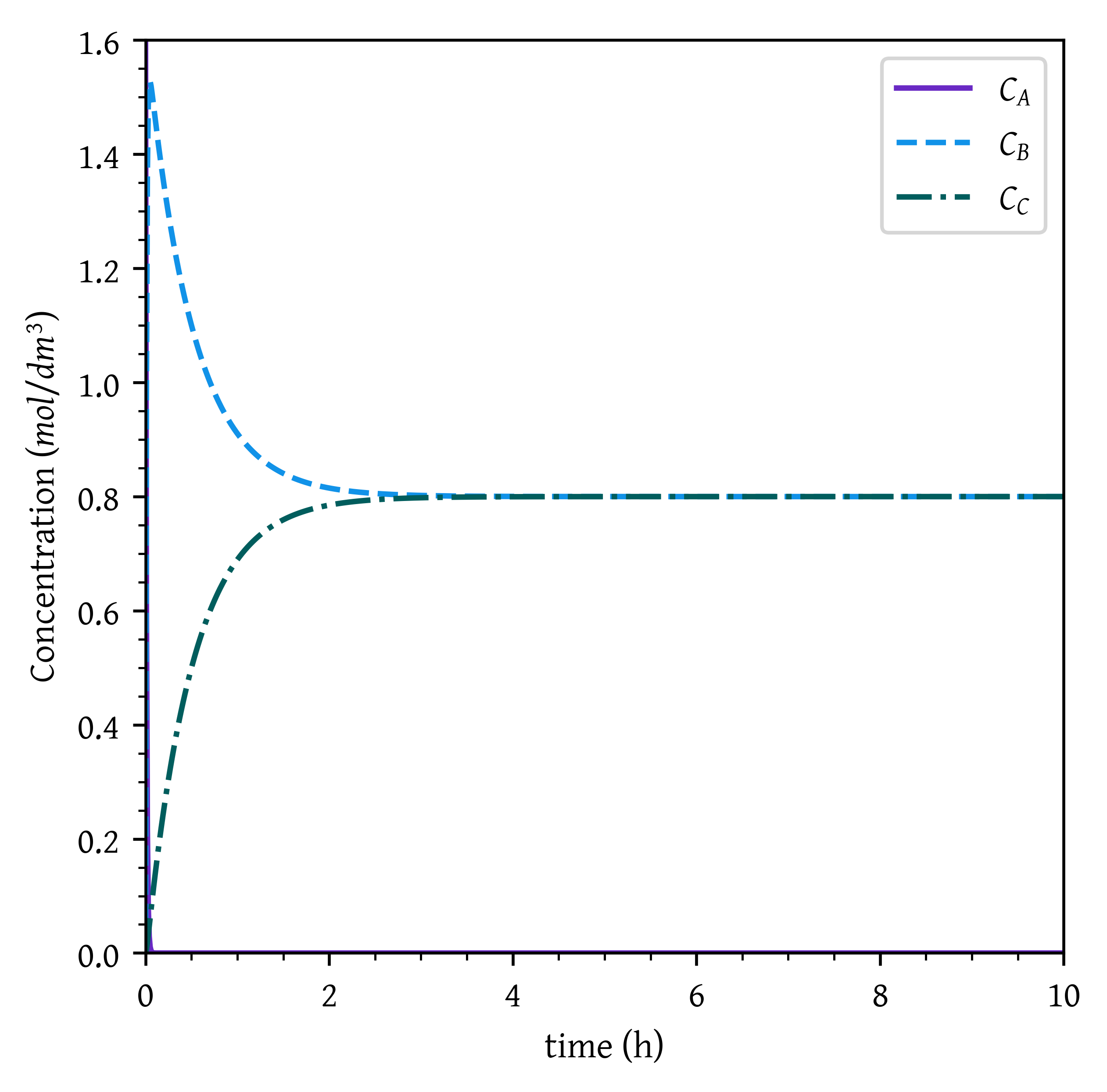
Since second reaction is reversible and K_{eq,2} = k_{2}/ k_{-2} = 1, a steady state (equilibrium) is achieved where C_B = C_C
k1 = 100
k2 = 1
km1 = 0
km2 = 0.25
# initial conditions
y0 = [ca0, 0, 0]
args = (k1, k2, km1, km2)
t_final = 10
sol = solve_ivp(batch_reactor_c, [0, t_final], y0, args=args, dense_output=True)
t = np.linspace(0,t_final, 1000)
ca, cb, cc = sol.sol(t)
plt.plot(t, ca, label='$C_A$')
plt.plot(t, cb, label='$C_B$')
plt.plot(t, cc, label='$C_C$')

plt.xlabel('time (h)')
plt.ylabel('Concentration ($mol/dm^3$)')

# Setting x and y axis limits
plt.xlim(0, t_final)
plt.ylim(0, ca0)

plt.legend()
plt.show()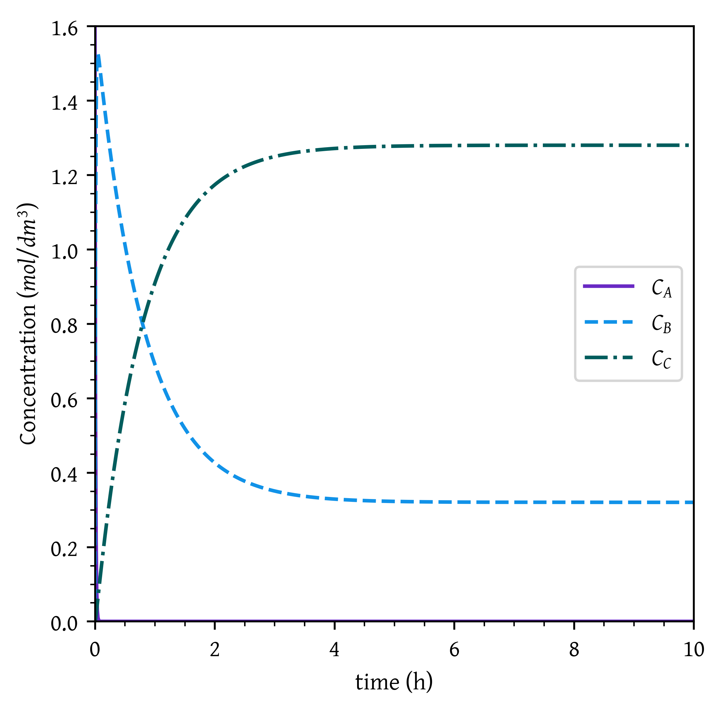
K_{eq} = k_{2}/ k_{-2} = 1/0.25 = 4, Therefore at equilibrium is achieved where C_C = 4 C_B
At equilibrium C_B = 0.32 mol/dm^3, C_C = 1.28 mol/dm^3
References
Fogler, H. Scott. 2016. Elements of Chemical Reaction Engineering. Fifth edition. Boston: Prentice Hall.
Citation
BibTeX citation:
@online{utikar2024,
  author = {Utikar, Ranjeet},
  title = {Solutions to Workshop 06: {Multiple} Reactions},
  date = {2024-03-24},
  url = {https://cre.smilelab.dev/content/workshops/06-multiple-reactions/solutions.html},
  langid = {en}
}
For attribution, please cite this work as:
Utikar, Ranjeet. 2024. “Solutions to Workshop 06: Multiple
Reactions.” March 24, 2024. https://cre.smilelab.dev/content/workshops/06-multiple-reactions/solutions.html.