Practice problem: Isothermal reactor design

CHEN3010/ CHEN5040: chemical reaction engineering

Introduction

Ethylene oxide (EO) ($\ce{C2H4O}$), also known as oxirane, is a colorless, flammable gas with a sweet, ether-like smell. EO is an important industrial chemical used primarily to make ethylene glycol (a key ingredient in antifreeze and polyester fiber) and other chemicals, such as surfactants, detergents, and solvents.

In 2022, global production of EO was nearly 28 millions of tons and s expected to grow at a steady CAGR of 4.07% during the forecast period until 2032. With a selling price of $1913 per tonne, the commercial value of EO is around $53 billion.

The primary route for EO production involves the direct vapor phase oxidation of ethylene in the presence of a silver catalyst:

$$\ce{C2H4 + 1/2 O2 -> C2H4O}$$

This reaction is highly exothermic and requires careful control to manage the risk of runaway reactions. The process typically involves a recovery stage to separate EO from water and other byproducts.

We want to design a reactor achieve a desired conversion of ethylene. Ethylene and oxygen (as air) are fed in stoichiometric proportions to a packed-bed reactor operated isothermally at 280 $^\circ C$. Ethylene is fed at a rate of 200 mol/s at a pressure of 10 atm (1013 kPa). It is proposed to use 10 banks of 25.4 mm diameter schedule 40 tubes packed with catalyst with 100 tubes per bank. Consequently, the molar flow rate to each tube is to be 0.2 mol/s.

The rate law for the reaction is

$$-r'_A = k P_A^{1/3} P_B^{2/3}$$

with k = 0.00392 $\frac{mol}{atm \ kg-cat\ s}$ at 260 $^\circ C$. The heat of reaction, $\Delta H$ is -106.7 kJ/mol and the activation energy, E is 69.49 kJ/mol.

Question 1: Reactor selection (5 marks)

In order to aid reactor design, laboratory experiments were performed at 260 °C to determine reaction rate at various ethylene conversions. The data is plotted in Figure 1.

We want to achieve 60% conversion of ethylene. What kind of reactor would you suggest? Why?

Figure 1: Rate data for oxidation of ethylene

Answer

Since this is a gas phase catalytic reaction a packed bed reactor would be ideal.

The $-r'_A vs. X$ graph is monotonously decreasing with conversion. Hence $(1/-r'_A) vs. X$ increases monotonically with conversion.

The amount of catalyst required is the area under the curve for a PBR and the area of rectangle with a width of $X_{exit}$ and height of $(F_{A0}/(-r'_A))_{exit}$.

For a monotonously increasing curve, catalyst weight using CSTR will always be higher than a PBR. Therefore PBR is preferred.

Question 2: Isobaric reactor design

1. Write correct mole balance equation(s) for flow reactors (CSTR, and PBR) in terms of conversion of ethylene. (5 marks)

2. Using the mole balances developed in (a), determine the weight of catalyst required to achieve 60% conversion in a PBR. Show your working by following the reaction engineering algorithm. State your assumptions if any. (10 marks)

Answer

(a) We write mole balance equations for the two flow reactors: CSTR, and PBR

1. CSTR $$W = \frac{F_{A0}X}{-r'_A}$$

2. PBR

   $$F_{A0}\frac{dX}{dW} = -r'_A$$

   and

   $$W = \int_{F_{A0}}^{F_A} \frac{dF_A}{r'_A}$$

   or

   $$W = F_{A0} \int_{0}^{X} \frac{dX}{r'_A}$$

(b) Isobaric reactor design

• Mole balance

  $$F_{A0}\frac{dX}{dW} = -r'_A \tag{1}$$

• Rate law

  $$-r'_A = k P_A^{1/3} P_B^{2/3} \tag{2}$$

  Where, $P_i = C_i RT_0$

  $$k(T) = k(T_0) e^{\frac{E}{R} \left( \frac{1}{T_0} - \frac{1}{T} \right)}$$

• Stoichiometry

  For isothermal, isobaric reactors $$C_j = \frac{C_{A0} (\Theta_j + \nu_j X)} {(1 + \epsilon X)} \tag{3}$$

  Reaction: $$\begin{aligned} \ce{C2H4 + 1/2 O2} & \ce{-> C2H4O} \\ \ce{A + 1/2 B } & \ce{-> C} \end{aligned}$$

• Combine

  Solve equations 1, 2, and 3 to obtain conversion as a function of catalyst weight.

• Evaluate

import numpy as np
from scipy.integrate import solve_ivp
import matplotlib.pyplot as plt

T = 280 + 273.15  # K
T0 = 260 + 273.15 # K
P0 = 10 # atm

k0 = 0.00392 #  mol/ (atm kg-cat s)

R = 0.082    # atm dm^3/ (mol K)
E = 69490    # J/mol

# It is usually a good idea to write k as a function of temperature. However,
# since we are simulating isothermal case, we just evaluate it. 
k = k0 * np.exp((E/8.314) * ((1/T0) - (1/T)))

fa0 = 0.2
fb0 = 0.5 * fa0
fc0 = 0 
fi0 = fb0 * (79/21)

ft0 = fa0 + fb0 + fc0 + fi0

thetaA = fa0/fa0
thetaB = fb0/fa0
thetaC = fc0/fa0
thetaI = fi0/fa0

ya0 = fa0/ft0
delta = -0.5
epsilon = ya0 * delta

pa0 = ya0 * P0
ca0 = pa0/(R * T)

• $k$ at 280 $^\circ C$

  k = 0.00392 $\frac{mol}{atm \ kg-cat\ s}$ at 260 $^\circ C$.

  $$k(T) = k(T_0) e^{\frac{E}{R} \left( \frac{1}{T_0} - \frac{1}{T} \right)}$$

  k at 280 $^\circ C$ = 0.00691 $\frac{mol}{atm \ kg-cat\ s}$

$\nu_A = -1; \nu_B = -1/2; \nu_C = 1$

Ethylene and oxygen are fed in stoichiometric proportions to a packed-bed. The oxygen is fed as air (21% O₂ and 79% N₂ (Inert)).

$F_{A0}$ = 0.20 mol/s

$F_{B0} = 0.5 F_{A0}$ = 0.10 mol/s

$F_{C0}$ = 0.00 mol/s

$F_{I0} = 0.5 \times (79/21)$ = 0.38 mol/s

$F_{T0}$ = 0.68 mol/s

$\Theta_i = F_{i0}/F_{A0}$: $\Theta_A$ = 1.00 , $\Theta_B$ = 0.50 , $\Theta_C$ = 0.00 , $\Theta_I$ = 1.88 mol/s.

$\delta = 1 - 1 - \frac{1}{2} = -\frac{1}{2}$

$y_{A0} = F_{A0}/ (F_{A0} + F_{B0})$ = 0.30.

$\epsilon = y_{A0} \delta$ = -0.15.

$P_{A0} = y_{A0} P_0$ = 2.96 atm

$C_{A0} = P_{A0} RT$ = 0.07 $mol/dm^3$.

def pbr(W, y, *args):
  X = y[0]

  fa0, ca0, thetaA, thetaB, nu_A, nu_B, epsilon, k = args

  ca = ca0 * (thetaA + nu_A * X)/ ( 1 + epsilon * X) 
  cb = ca0 * (thetaB + nu_B * X)/ ( 1 + epsilon * X) 

  pa = ca *(R * T) 
  pb = cb *(R * T)  

  rate = k * pa**(1/3) * pb**(2/3)

  dXdW = rate/ fa0

  return [dXdW]

nu_A = -1
nu_B = -0.5

# Solve the pbr model
W = 25 # kg

# initial conditions
y0 = [0]

system_args = (fa0, ca0, thetaA, thetaB, nu_A, nu_B, epsilon, k)

sol = solve_ivp(pbr, [0, W], y0, args=system_args, dense_output=True)

w = np.linspace(0,W, 1000)
X = sol.sol(w)[0]

x_final = X[X > 0.6][0]
w_final = w[X > 0.6][0]

Weight of catalyst required to achieve a conversion of 60%, W = 13.51 kg. The final conversion is X = 0.60.

Question 3: Effect of pressure drop (20 marks)

As this is a gas phase reaction carried out in a PBR, there is a significant pressure drop. The properties of the reacting fluid are to be considered identical to those of air at this temperature and pressure. The density of the 6.35 mm catalyst particles is 1925 $kg/m^3$, the bed void fraction is 0.45, and the gas density is 16 $kg/m^3$. For these catalyst properties, the pressure drop parameter $\alpha$ is 0.0367 $1/kg$

1. How will the equations change when you consider pressure drop? (4 marks)

2. Draw the profiles of concentrations of reactants and products, conversion, volumetric flow rate ratio ($\upsilon/\upsilon_0$), and pressure ratio ($P/P_0$) as a function of catalyst weight. (12 marks)

3. Estimate the catalyst weight required to achieve 60% conversion considering pressure drop. Compare the results with those obtained in question 2. (4 marks)

Answer

a. How will the equations change when you consider pressure drop?

• Mole balance

  No change

  $$F_{A0}\frac{dX}{dW} = -r'_A \tag{4}$$

• Rate law

  No change

  $$-r'_A = k P_A^{1/3} P_B^{2/3} \tag{5}$$

  Where, $P_i = C_i RT_0$

  $$k(T) = k(T_0) e^{\frac{E}{R} \left( \frac{1}{T_0} - \frac{1}{T} \right)}$$

• Stoichiometry

  The reator is no more isobaric

  For isothermal reactors

  $$\frac{\upsilon}{\upsilon_0} = (1 + \epsilon X) \left( \frac{P_0}{P}\right)$$

  $$C_j = \frac{C_{A0} (\Theta_j + \nu_j X)} {(1 + \epsilon X)} \left( \frac{P}{P_0} \right) \tag{6}$$

  Reaction: $$\begin{aligned} \ce{C2H4 + 1/2 O2} & \ce{-> C2H4O} \\ \ce{A + 1/2 B } & \ce{-> C} \end{aligned}$$

• Pressure drop

  $$\frac{dp}{dW} = -\frac{\alpha}{2p} \left( 1 + \epsilon X \right) \tag{7}$$

  Where: $p = P/P_0$

• Combine

  Solve equations 4, 5, 6, and 7 to obtain conversion as a function of catalyst weight.

• Evaluate

def pbr_with_pressure_drop(W, y, *args):
  
  X,p = y
  fa0, ca0, thetaA, thetaB, nu_A, nu_B, epsilon, k, alpha = args
  
  ca = ca0 * (thetaA + nu_A * X)/ ( 1 + epsilon * X) * p 
  cb = ca0 * (thetaB + nu_B * X)/ ( 1 + epsilon * X) * p

  pa = ca * R * T 
  pb = cb * R * T  

  rate = k * pa**(1/3) * pb**(2/3)
  
  dXdW = rate/ fa0
  
  dpdW = - alpha * (1 + epsilon * X) / (2 * p)

  return [dXdW, dpdW]

nu_A = -1
nu_B = -0.5
nu_C = 1
nu_I = 0

# Solve the pbr model
W = 25 # kg

# initial conditions
# at W = 0 , X = 0; p = 1
y0 = [0, 1]

alpha = 0.0367
system_args = (fa0, ca0, thetaA, thetaB, nu_A, nu_B, epsilon, k, alpha)

sol = solve_ivp(
    pbr_with_pressure_drop, 
    [0, W], 
    y0, 
    args=system_args, 
    dense_output=True
)

w = np.linspace(0,W, 1000)
X = sol.sol(w)[0]
p = sol.sol(w)[1]

x_final_2 = X[X > 0.6][0]
w_final_2 = w[X > 0.6][0]

b. Draw the profiles

# Concentrations
# C_j = C_A0 * (Theta_j + nu_j * X) * p/ (1 + epsilon *X)
ca = lambda X, p: ca0 * (thetaA + nu_A * X) * p / (1 + epsilon * X)
cb = lambda X, p: ca0 * (thetaB + nu_B * X) * p / (1 + epsilon * X)
cc = lambda X, p: ca0 * (thetaC + nu_C * X) * p / (1 + epsilon * X)
ci = lambda X, p: ca0 * (thetaI + nu_I * X) * p / (1 + epsilon * X)

# volumetric flow rate ratio
# v/v0 = (1 + epsilon * X) * P_0/P = (1 + epsilon * X)/p
vv0 = lambda X, p: (1 + epsilon * X)/p

# Set up graph

x_p = X[X < 0.6]
p_p = p[X < 0.6]
w_p = w[X < 0.6]

ca_p = ca(x_p, p_p)
cb_p = cb(x_p, p_p)
cc_p = cc(x_p, p_p)
ci_p = ci(x_p, p_p)

vv0_p = vv0(x_p, p_p)

plt.plot(w_p, ca_p, label='$C_A$')
plt.plot(w_p, cb_p, label='$C_B$')
plt.plot(w_p, cc_p, label='$C_C$')
plt.plot(w_p, ci_p, label='$C_I$')

plt.xlabel('Catalyst weight (kg)')
plt.ylabel('Concentration $mol/dm^3$')

# Setting x and y axis limits
plt.xlim(0, np.ceil(w_final_2))
plt.ylim(0, 0.14)

plt.legend(loc='upper right')

ax = plt.gca()
ax.grid(which='major', linestyle='-', linewidth='0.5', color='gray')

plt.show()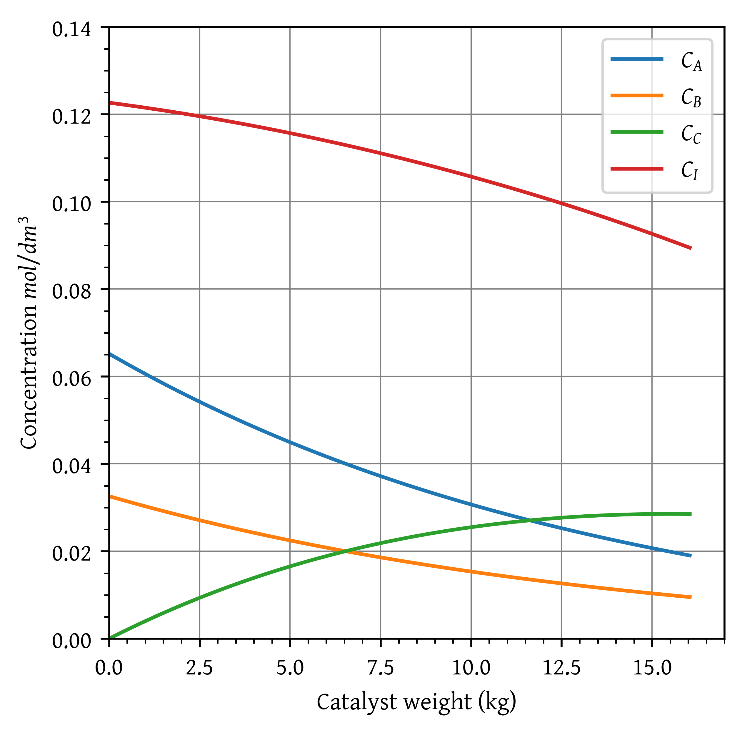

Figure 2: Concentration profile (2 marks)

plt.plot(w_p, x_p, label='conversion ($X$)')
plt.plot(w_p, vv0_p, label='$\\upsilon/\\upsilon_0 (f)$')
plt.plot(w_p, p_p, label='$P/P_0 (p)$')

plt.xlabel('Catalyst weight (kg)')
plt.ylabel('$X, f, p$')

# Setting x and y axis limits
plt.xlim(0, np.ceil(w_final_2))
plt.ylim(0, 1.4)

plt.legend()

ax = plt.gca()
ax.grid(which='major', linestyle='-', linewidth='0.5', color='gray')
plt.show()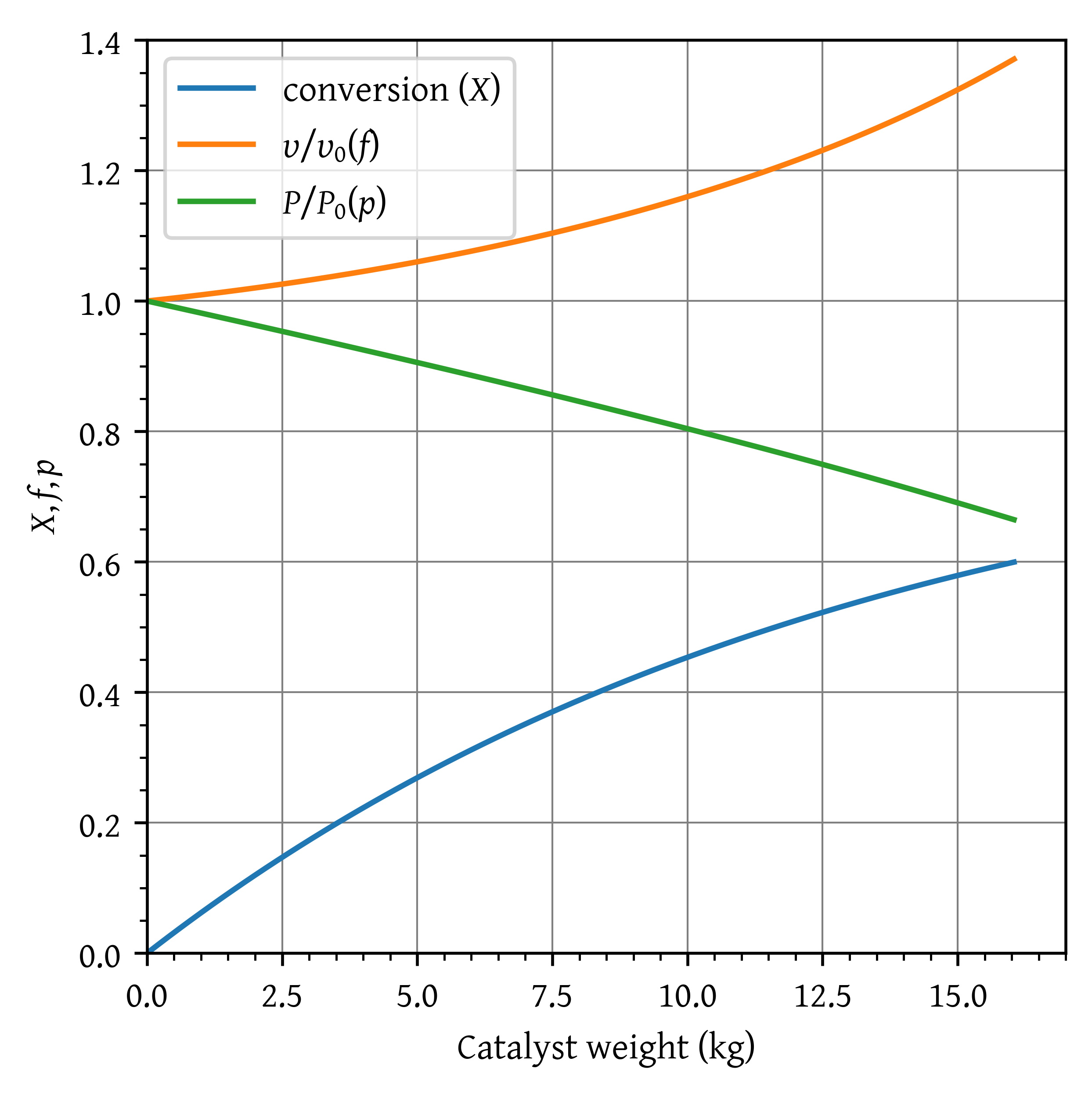

Figure 3: Conversion, volumetric flow ratio, pressure ratio profile (4 marks)

• half marks for essentially correct procedure but wrong answers.

c. Estimate the catalyst weight required to achieve 60% conversion

Weight of catalyst required to achieve a conversion of 60%, W = 16.07 kg. The final conversion is X = 0.60.

As the presesure decreases within the reactor, the cocentration (and consequently the rate) decreases. This results into lower conversion for the same catalyst weight.

For the isobaric case, to achieve a conversion of 0.60, we needed 13.51 kg catalyst. If we used this catalyst weight to manufacture our reactor, the real life conversion would have been 0.55 and our reactor would severely underperform.