You can use textbooks, the resources provided during class/ workshop etc. to answer the questions.
The portfolio task is made available in both pdf format and as a print.
You are free to choose a solution technique. It is not required that you use the provided python code to answer the questions. You can use any tool (pen and paper, excel, … ) and any technique (graphical, numerical, analytical) that you are comfortable with.
Irrespective of your solution method, you are expected to write your answers on to the printed question paper provided. This is what gets marked.
The portfolio will take place during designated time slot communicated earlier by the unit coordinator. Please refer to the portfolio schedule on blackboard for the portfolio dates and topics.
The tasks will be a mix of theory questions, short calculation type and long numerical examples.
You have 50 minutes to complete the tasks in the portfolio.
The portfolios will be marked immediately after completion by your peers using a provided marking rubric.
The portfolios will be collected by the instructors to verify peer marking and record the marks. You will receive your portfolio back within a week.
When you are required to upload the portfolio answers on to blackboard:
Save your report as a pdf file.
Rename the file as STUDENTID_Portfolio_x.pdf (Where STUDENTID is your student ID, and x is the portfolio number) and
Upload it using assessment submission link on blackboard.
Academic Integrity
Academic integrity at its core is about honesty and responsibility and is fundamental to Curtin’s expectations of you. This means that all of your work at Curtin should be your own and it should be underpinned by integrity, which means to act ethically, honestly and with fairness.
As a Curtin student you are part of an academic community and you are asked to uphold the University’s Code of Conduct, principles of academic integrity, and Curtin’s five core values of integrity, respect, courage, excellence and impact during your studies.
You are also expected to uphold the Student Charter and recognize that cheating, plagiarism collusion, and falsification of data and other forms of academic dishonesty are not acceptable.
The ethylene epoxydation is to be carried out using a cesium-doped silver catalyst in a packed-bed reactor.
The feed enters the reactor at 250 °C and a pressure of 2 atm. The reactor contains 3.5 kg of catalyst.
A pulse test was carried out at two different flow rates (\upsilon) to assess the residence time distribution in the reactor.
The concentration of the tracer was measured at the outlet is reported in Table 1. The data is also available in Excel .csv format at portfolio_8_data.csv.
Table 1: Tracer concentration at outlet
\upsilon = 0.6 \, \text{dm}^3/\text{s}
\upsilon = 0.2 \, \text{dm}^3/\text{s}
Time (s)
Tracer Concentration (ppm)
Time (s)
Tracer Concentration (ppm)
————–
——————————————
————–
——————————————
0
0
0
0
0.5
8
0.5
0
1
640
1
0
1.5
951
1.5
0
2
495
2
0
2.5
215
2.5
61
3
103
3
270
4
34
3.5
475
5
11
4
605
6
7
4.5
659
7
0
5
614
6
396
7
227
8
130
9
80
10
47
12
26
14
12
16
0
Questions
What are the mean residence time t_m, the variance, \sigma^2, and mean internal age \alpha_m? (6 marks)
t_m
\sigma^2
\alpha_m
\upsilon = 0.6 \, \text{dm}^3/\text{s}
1.752 s
0.620 s^2
1.105 s
\upsilon = 0.2 \, \text{dm}^3/\text{s}
5.515 s
4.44 s^2
1.058 s
Comment on the results obtained (4 marks)
Mean residence time increases as volumetric flow rate is decreased (material spends more time in the reactor)
At high volumetric flow rate, variance is lower, indicating that the flow behavior is more akin to plug flow. At lower volumetric flow rate, higher dispersion is observed resulting in a bigger spread of the RTD curve.
The mean internal age is about the same for both the flow rates.
For \upsilon = 0.2 \, \text{dm}^3/\text{s}, what fraction of the material spends between 4 and 6 s in the reactor? (2 marks)
fraction_4_to_6, _ = quad(et_interp, 4, 6)
0.465
For \upsilon = 0.6 \, \text{dm}^3/\text{s}, what fraction of the material spends less than 2 s in the reactor? (2 marks)
fraction_0_to_2, _ = quad(et_interp, 0, 2)
0.714
For \upsilon = 0.6 \, \text{dm}^3/\text{s} what fraction of the material spends longer than 1 s in the reactor? (2 marks)
If you were to repeat the experiments, what would you do differently? (2 marks)
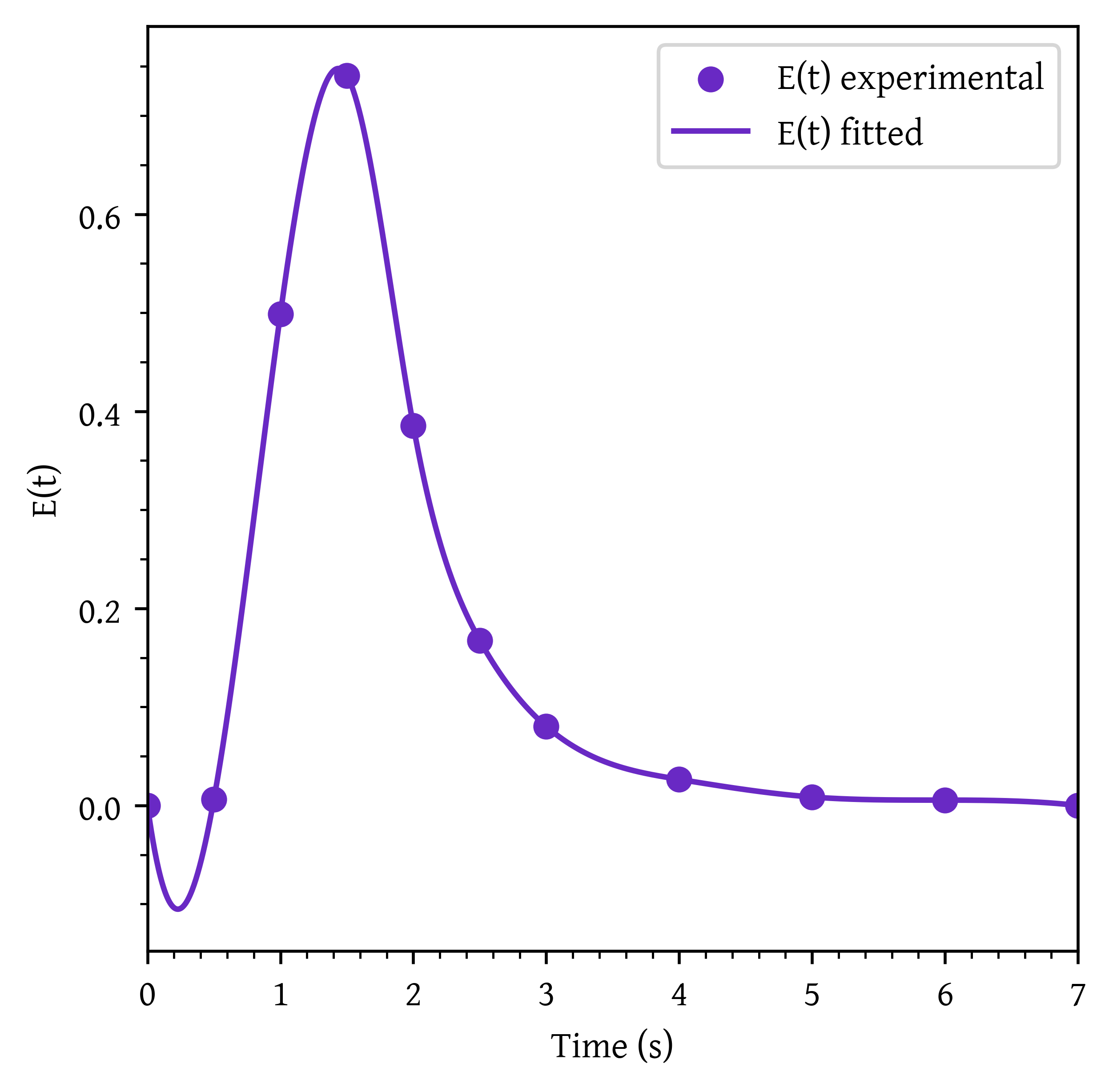
For high flow rate case, try and get more data in the first 1.5 s of experiment as the interpolation results in negative values for the first 0.5s.
Appendix
The code is also available as ipython notebook. Download the file portfolio_8.ipynb from blackboard. Open Google colab. From menu, click on File > Upload notebook. Upload the downloaded file and modify as per needed.
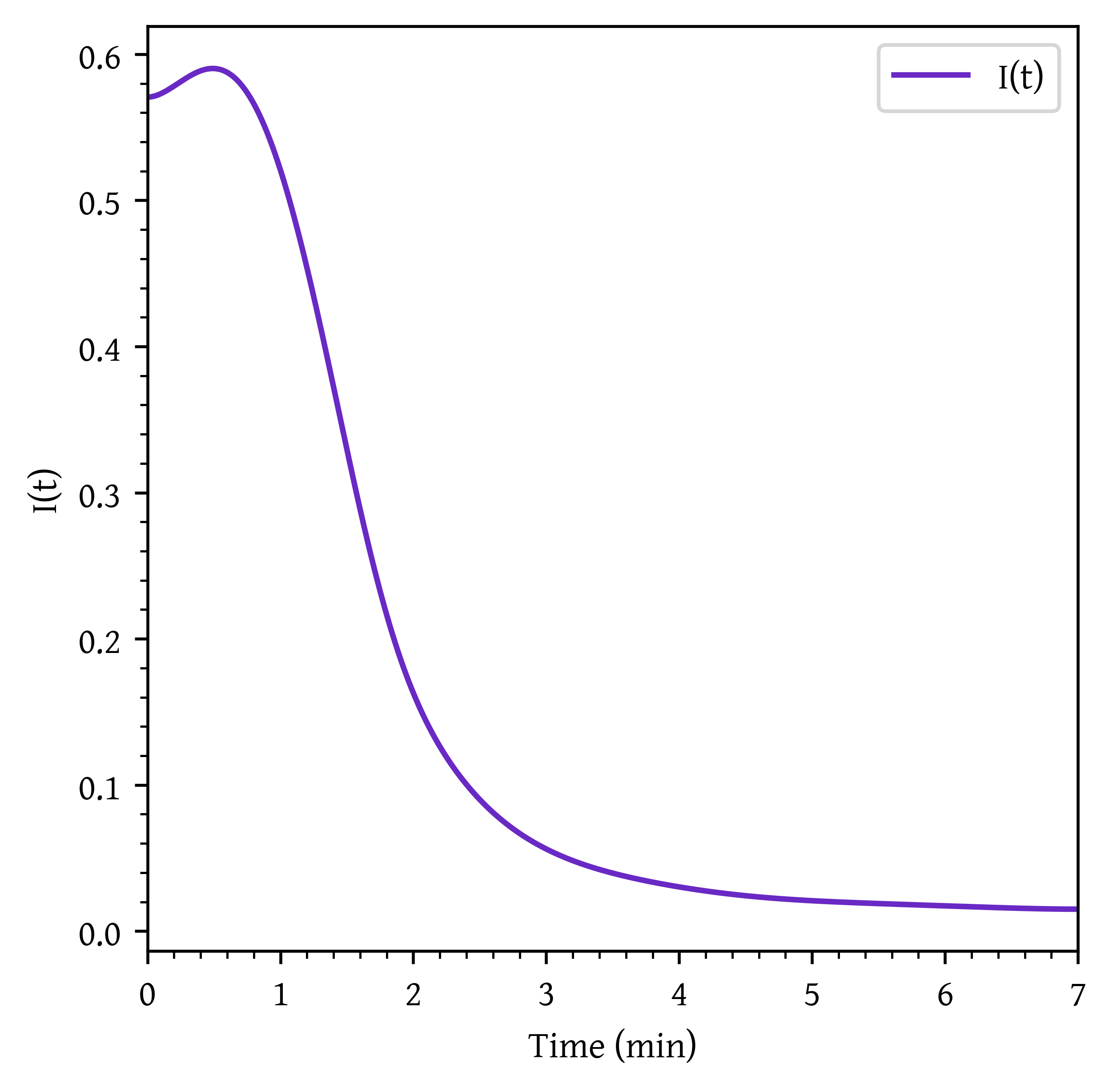
import matplotlib.pyplot as pltimport numpy as npfrom scipy.integrate import quadfrom scipy.interpolate import interp1dfrom scipy.interpolate import PchipInterpolator # Given datacolumn_names = ["time (s)", "Tracer concentration (ppm)"]data_v_p6 = [ # Data for v = 0.6 dm^3/s (0, 0), (0.5, 8), (1, 640), (1.5, 951), (2, 495), (2.5, 215), (3, 103), (4, 34), (5, 11), (6, 7), (7, 0),]data_v_p6 = np.array( data_v_p6, dtype={"names": column_names, "formats": [float, float]})data_v_p2 = [ # Data for v = 0.2 dm^3/s (0, 0), (0.5, 0), (1, 0), (1.5, 0), (2, 0), (2.5, 61), (3, 270), (3.5, 475), (4, 605), (4.5, 659), (5, 614), (6, 396), (7, 227), (8, 130), (9, 80), (10, 47), (12, 26), (14, 12), (16, 0),]data_v_p2 = np.array( data_v_p2, dtype={"names": column_names, "formats": [float, float]})# working with data for v = 0.6 dm^3/s# replace data_v_p6 with data_v_p2 to change the data set# to v = 0.2 dm^3/s (also need to change Q)# Flow rateQ =0.6# dm^3/mint = data_v_p6["time (s)"]c = data_v_p6["Tracer concentration (ppm)"]# Normalize concentration to calculate E(t)integral_c = np.trapz(c, t)et = c / integral_c# Interpolation functionset_interp = interp1d(t, et, kind="cubic", fill_value="extrapolate")# Better interpolation# et_interp = PchipInterpolator(t, et, extrapolate=True)# Define cumulative distribution F(t)def f_interp(t):return np.array([quad(et_interp, 0, ti, limit=1000)[0] for ti in np.atleast_1d(t)])# Mean residence time functiontau_func =lambda t: t * et_interp(t)# Variance functionvariance_func =lambda t, tm: (t - tm) **2* et_interp(t)# Skewness functionskewness_func =lambda t, tm: (t - tm) **3* et_interp(t)# Calculate mean residence time (t_m)tau, _ = quad(tau_func, 0, np.max(t))# Calculate variance (σ²)variance, _ = quad(variance_func, 0, np.max(t), args=(tau,))# Calculate skewness (sigma = variance**0.5fac =1.0/ (sigma**1.5)integral, _ = quad(skewness_func, 0, np.max(t), args=(tau,))skewness = fac * integral# Calculate specific time fractions# uncomment and adopt the following line as per required# When you need to find integral till infinity,# in place of infinity use np.max(t)# fraction_2_to_4, _ = quad(et_interp, 2, 4)fraction_4_to_6, _ = quad(et_interp, 4, 6)fraction_0_to_2, _ = quad(et_interp, 0, 2)fraction_1_to_inf, _ = quad(et_interp, 1, np.max(t))internal_age =lambda t, tm: (1/ tm) * (1- f_interp(t))mean_internal_age, _ = quad(lambda t: internal_age(t, tau), 0, np.max(t))# Reactor volume calculationvolume = Q * taut_plot = np.linspace(0, np.max(t), 1000)et_plot = et_interp(t_plot)plt.scatter(t, et, label='E(t) experimental')plt.plot(t_plot, et_plot, label='E(t) fitted')plt.xlabel('Time (s)')plt.ylabel('E(t)')plt.xlim(np.min(t_plot), np.max(t_plot))plt.legend()plt.show()it_plot = internal_age(t_plot, tau)plt.plot(t_plot, it_plot, label='I(t)')plt.xlabel('Time (min)')plt.ylabel('I(t)')plt.xlim(np.min(t_plot), np.max(t_plot))plt.legend()plt.show()
Citation
BibTeX citation:
@online{2024,
  author = {},
  title = {Portfolio 08: {Distribution} of Residence Times},
  date = {2024-05-14},
  url = {https://cre.smilelab.dev/content/portfolio/08-distribution-of-residence-time/portfolio-08-answers.html},
  langid = {en}
}