In class activity: Distribution of residence time

Lecture notes for chemical reaction engineering

Finding the RTD function by experiment

Plot the C-curve and E-curve for a response to a pulse input into a reactor given in Table 1.

Table 1: Concentration-Time Data

t(min)	0.00	5.00	10.00	15.00	20.00	25.00	30.00	35.00	40.00
C_{\text{tracer}} \ (g/dm^3)	0.00	4.00	6.00	7.00	5.00	3.00	2.00	1.00	0.00

Solution

import numpy as np
import matplotlib.pyplot as plt
from scipy.integrate import quad
from scipy.interpolate import interp1d

data_p1 = np.array([
    (0, 0), (5, 4), (10, 6), (15, 7), (20, 5),
    (25, 3), (30, 2), (35, 1), (40, 0)
], dtype=[('t(min)', float), ('$C_{tracer} \\ (g/dm^3)$', float)])

t = data_p1["t(min)"]
c = data_p1["$C_{tracer} \\ (g/dm^3)$"]

c_interp = interp1d(t, c, kind="cubic", fill_value="extrapolate")

# Plot C(t)
t_plot = np.linspace(0, np.max(t), 500)
c_plot = c_interp(t_plot)

plt.scatter(t, c, label='C(t) experimental')
plt.plot(t_plot, c_plot, label='C(t) fitted')
plt.xlabel('Time (min)')
plt.ylabel('$C_{tracer} \\ (g/dm^3)$')
plt.xlim(np.min(t_plot), np.max(t_plot))
plt.ylim(0,10)
plt.legend()
plt.show()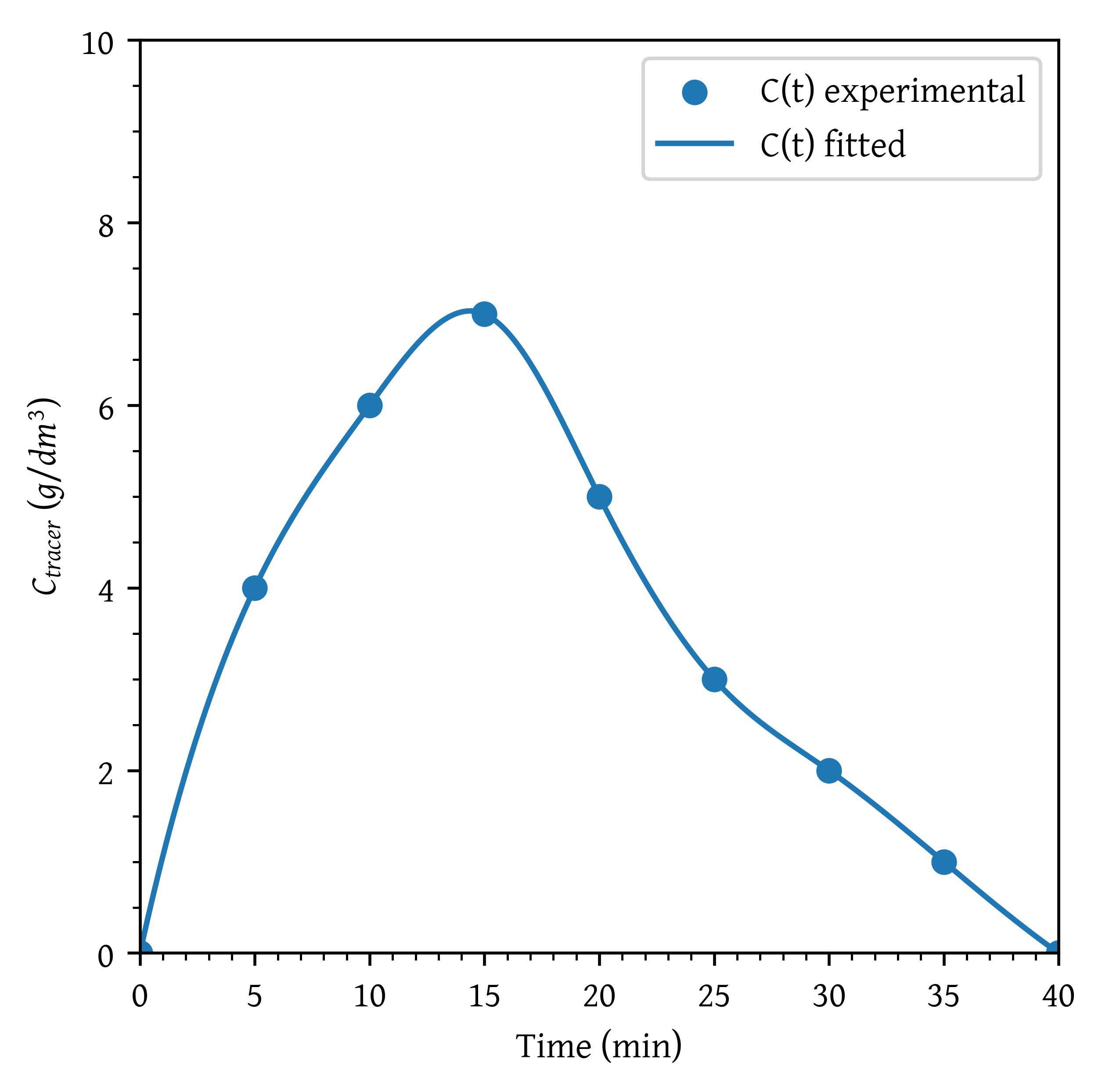

Figure 1: C Curve

# Normalize concentration to calculate E(t)
integral_c = np.trapz(c, t)
et = c / integral_c

et_interp = interp1d(t, et, kind="cubic", fill_value="extrapolate")

# Plot C(t)
et_plot = et_interp(t_plot)

plt.scatter(t, et, label='E(t) experimental')
plt.plot(t_plot, et_plot, label='E(t) fitted')
plt.xlabel('Time (min)')
plt.ylabel('E(t)')
plt.xlim(np.min(t_plot), np.max(t_plot))
plt.ylim(0,0.06)
plt.legend()
plt.show()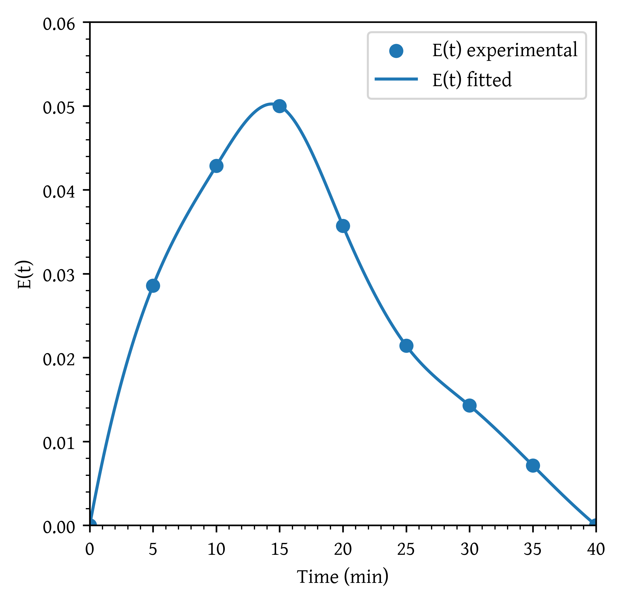

Figure 2: E Curve

Constructing the C(t) and E(t) Curves

A sample of the tracer hytane at 320 K was injected as a pulse into a reactor, and the effluent concentration was measured as a function of time, resulting in the data shown in Table 2

Table 2: Concentration-Time Data

t(min)	0.00	1.00	2.00	3.00	4.00	5.00	6.00	7.00	8.00	9.00	10.00	12.00	14.00
C (g/m^3)	0.00	1.00	5.00	8.00	10.00	8.00	6.00	4.00	3.00	2.20	1.50	0.60	0.00

The measurements represent the exact concentrations at the times listed and not average values between the various sampling tests.

• Construct a figure showing the tracer concentration C(t) as a function of time.
• Construct a figure showing E(t) as a function of time.

Solution

import numpy as np
import matplotlib.pyplot as plt
from scipy.integrate import quad
from scipy.interpolate import interp1d

data_p2 = np.array([
    (0, 0), (1, 1), (2, 5), (3, 8), (4, 10),
    (5, 8), (6, 6), (7, 4), (8, 3), (9, 2.2),
    (10, 1.5), (12, 0.6), (14, 0)
], dtype=[('t(min)', float), ('C ($g/m^3$)', float)])

t = data_p2["t(min)"]
c = data_p2["C ($g/m^3$)"]

c_interp = interp1d(t, c, kind="cubic", fill_value="extrapolate")

# Plot C(t)
t_plot = np.linspace(0, np.max(t), 500)
c_plot = c_interp(t_plot)

plt.scatter(t, c, label='C(t) experimental')
plt.plot(t_plot, c_plot, label='C(t) fitted')
plt.xlabel('Time (min)')
plt.ylabel('$C_{tracer} \\ (g/dm^3)$')
plt.xlim(np.min(t_plot), np.max(t_plot))
plt.legend()
plt.show()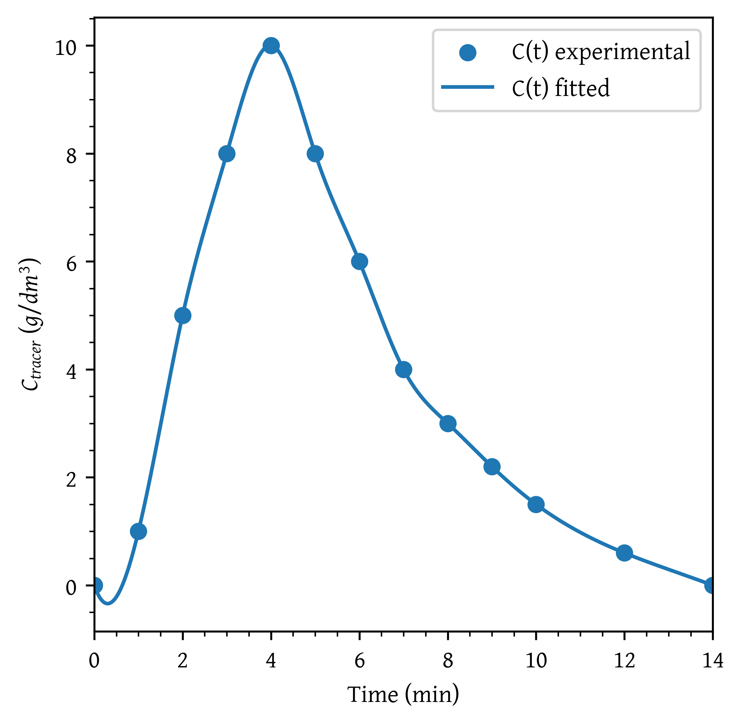

Figure 3: C Curve

# Normalize concentration to calculate E(t)
integral_c = np.trapz(c, t)
et = c / integral_c

et_interp = interp1d(t, et, kind="cubic", fill_value="extrapolate")

# Plot C(t)
et_plot = et_interp(t_plot)

plt.scatter(t, et, label='E(t) experimental')
plt.plot(t_plot, et_plot, label='E(t) fitted')
plt.xlabel('Time (min)')
plt.ylabel('E(t)')
plt.xlim(np.min(t_plot), np.max(t_plot))
plt.legend()
plt.show()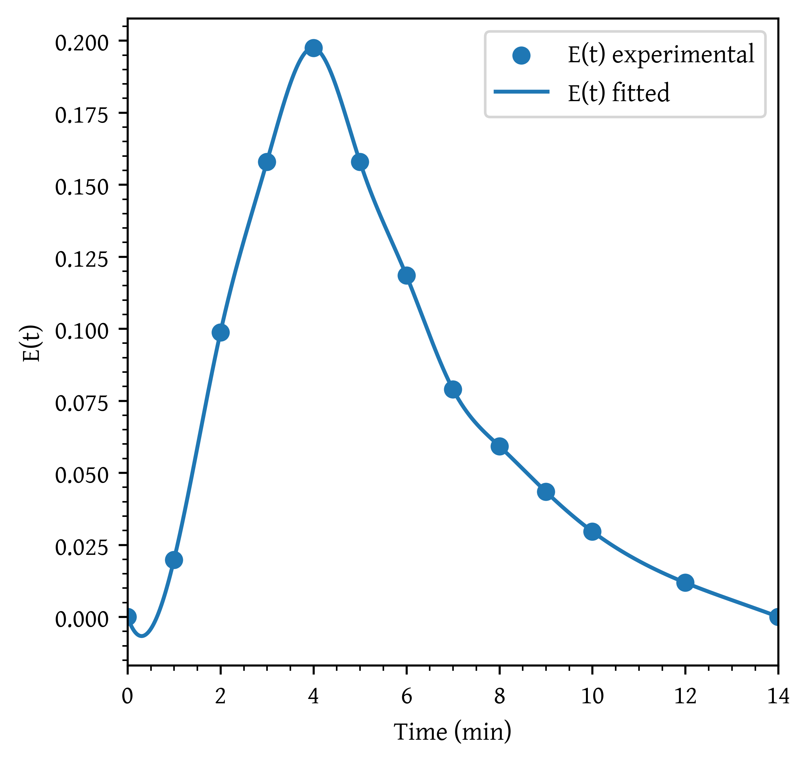

Figure 4: E Curve

The interpolation results in unrealistic values for C(t) and E(t) between 0 and 1. An undershoot is observed resulting in negative concentrations.

The interp1d function with kind='cubic' performs cubic spline interpolation, which can sometimes result in overshooting, especially when the data points have steep slopes or sharp changes. Cubic splines are designed to produce smooth curves, but this smoothness can lead to values that fall below zero in regions where the slope changes rapidly.

To avoid the cubic interpolation returning negative values, one can use the scipy.interpolate.PchipInterpolator instead of interp1d. The PchipInterpolator uses piecewise cubic Hermite interpolating polynomials (PCHIP stands for Piecewise Cubic Hermite Interpolating Polynomial) which preserve the shape and monotonicity of the data. This ensures that the interpolated values are monotonic and do not overshoot, which helps in avoiding negative values for this type of data.

from scipy.interpolate import PchipInterpolator

c_interp = PchipInterpolator(t, c, extrapolate=True)
et_interp = PchipInterpolator(t, et, extrapolate=True)

c_plot = c_interp(t_plot)
et_plot = et_interp(t_plot)

# Plot side by side
fig, (ax1, ax2) = plt.subplots(1, 2, figsize=(12, 5))

# Plot C(t)
ax1.scatter(t, c, label='C(t) experimental')
ax1.plot(t_plot, c_plot, label='C(t) fitted')
ax1.set_xlabel('Time (min)')
ax1.set_ylabel('$C_{tracer} \\ (g/dm^3)$')
ax1.set_xlim(np.min(t_plot), np.max(t_plot))
ax1.legend()

# Plot E(t)
ax2.scatter(t, et, label='E(t) experimental')
ax2.plot(t_plot, et_plot, label='E(t) fitted')
ax2.set_xlabel('Time (min)')
ax2.set_ylabel('E(t)')
ax2.set_xlim(np.min(t_plot), np.max(t_plot))
ax2.legend()

plt.tight_layout()
plt.show()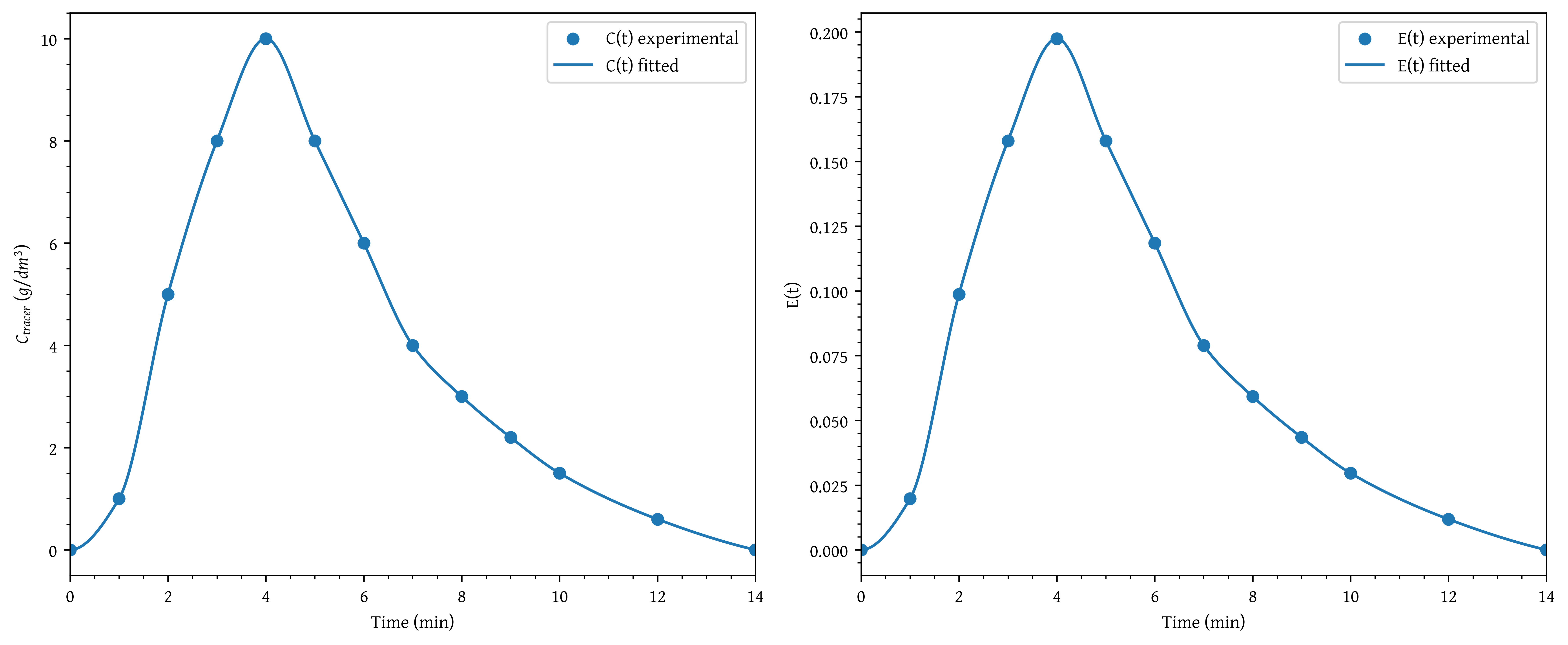

Figure 5: C and E Curve with proper interpolation

Mean Residence Time and Variance Calculations

Using the data given in Table 2 in the previous problem

• Construct the F(t) curve.
• Calculate the mean residence time, t_m.
• Calculate the variance about the mean, \sigma^2.
• Calculate the fraction of fluid that spends between 3 and 6 minutes in the reactor.
• Calculate the fraction of fluid that spends 2 minutes or less in the reactor.
• Calculate the fraction of the material that spends 3 minutes or longer in the reactor.

Solution

# Define cumulative distribution F(t)
def f_interp(t):
    return np.array([quad(et_interp, 
                          0, 
                          ti, 
                          limit=1000)[0] 
        for ti in np.atleast_1d(t)])

# Mean residence time function
tau_func = lambda t: t * et_interp(t)

# Variance function
variance_func = lambda t, tm: (t - tm) ** 2 * et_interp(t)

# Skewness function
skewness_func = lambda t, tm: (t - tm) ** 3 * et_interp(t)

# Calculate mean residence time (t_m)
tau, _ = quad(tau_func, 0, np.max(t))

# Calculate variance (σ²)
variance, _ = quad(variance_func, 0, np.max(t), args=(tau,))

# Calculate skewness (
sigma = variance**0.5
fac = 1.0 / (sigma**1.5)
integral, _ = quad(skewness_func, 0, np.max(t), args=(tau,))
skewness = fac * integral

f_plot = f_interp(t_plot)

plt.plot(t_plot, f_plot, label='F(t)')
plt.xlabel('Time (min)')
plt.ylabel('F(t)')
plt.xlim(np.min(t_plot), np.max(t_plot))
plt.ylim(0,1)
plt.legend()
plt.show()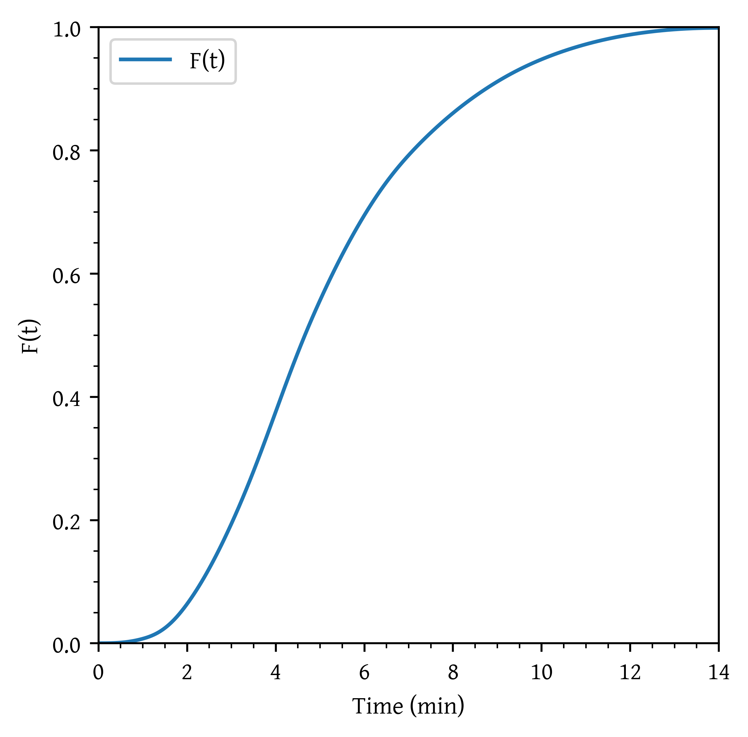

Figure 6: Cumulative distribution F(t)

# Calculate specific time fractions
fraction_3_to_6, _ = quad(et_interp, 3, 6)
fraction_below_2, _ = quad(et_interp, 0, 2)
fraction_above_3, _ = quad(et_interp, 3, np.max(t))

Mean Residence Time tau: \approx 5.126 min.

Variance \sigma^2: \approx 6.096 min^2

Skewness s^3: \approx 3.178 min^3

Specific Time Fractions:

Fraction of material that spends between 3 and 6 minutes: \approx 0.501

Fraction of material that spends less than 2 minutes: \approx 0.063

Fraction of material that spends longer than 3 minutes: \approx 0.805

Step experiment

A step experiment is made on a reactor at C_{in} ( t \ge 0 ) = 0.5 \ mol/dm^3. The results are as given in Table 3.

Table 3: Concentration-Time data from step experiment

t (min)	0.00	1.00	2.00	3.00	4.00	5.00	6.00	7.00	8.00
C_{out} (mol/L)	0.00	0.00	0.10	0.20	0.30	0.40	0.50	0.50	0.50

Plot the Concentration - time curve, F(t) curve and E(t) curve.

Solution

data_p4 = np.array([
    (0, 0), (1, 0), (2, 0.1), (3, 0.2), (4, 0.3),
    (5, 0.4), (6, 0.5), (7, 0.5), (8, 0.5)
], dtype=[('t (min)', float), ('$C_{out} (mol/L)$', float)])

t = data_p4["t (min)"]
c = data_p4["$C_{out} (mol/L)$"]

c_interp = interp1d(t, c, kind="linear", fill_value="extrapolate")

# Plot C(t)
t_plot = np.linspace(0, np.max(t), 500)
c_plot = c_interp(t_plot)

plt.scatter(t, c, label='C(t) experimental')
plt.plot(t_plot, c_plot, label='C(t) fitted')
plt.xlabel('Time (min)')
plt.ylabel('$C_{tracer} \\ (g/dm^3)$')
plt.xlim(np.min(t_plot), np.max(t_plot))
plt.legend()
plt.show()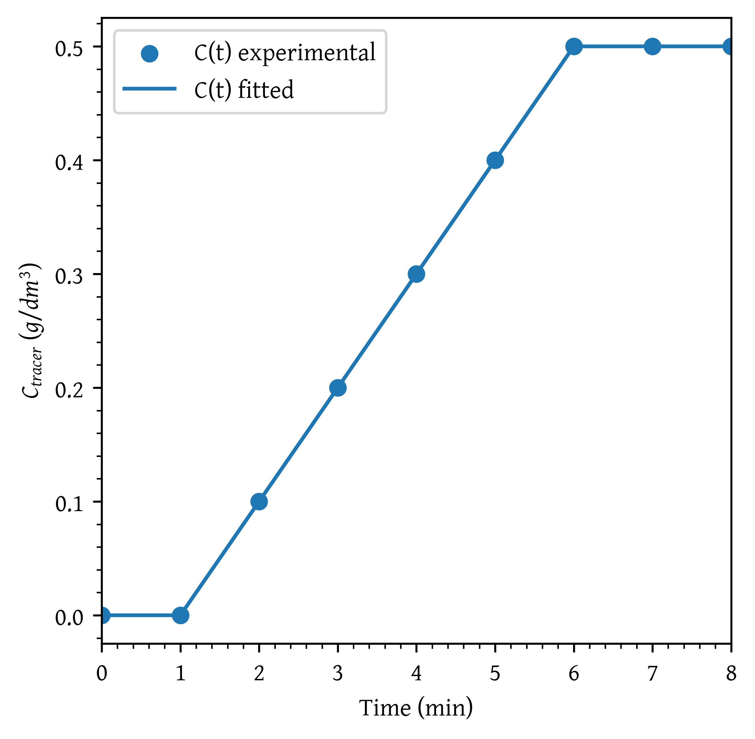

Figure 7: C Curve

C0 = 0.5 # mol/l
f = c/C0
f_interp = interp1d(t, f, kind="linear", fill_value="extrapolate")

f_plot = f_interp(t_plot)

plt.scatter(t, f, label='F(t) experimental')
plt.plot(t_plot, f_plot, label='F(t) fitted')
plt.xlabel('Time (min)')
plt.ylabel('F(t)')
plt.xlim(np.min(t_plot), np.max(t_plot))
plt.ylim(0,1)
plt.legend()
plt.show()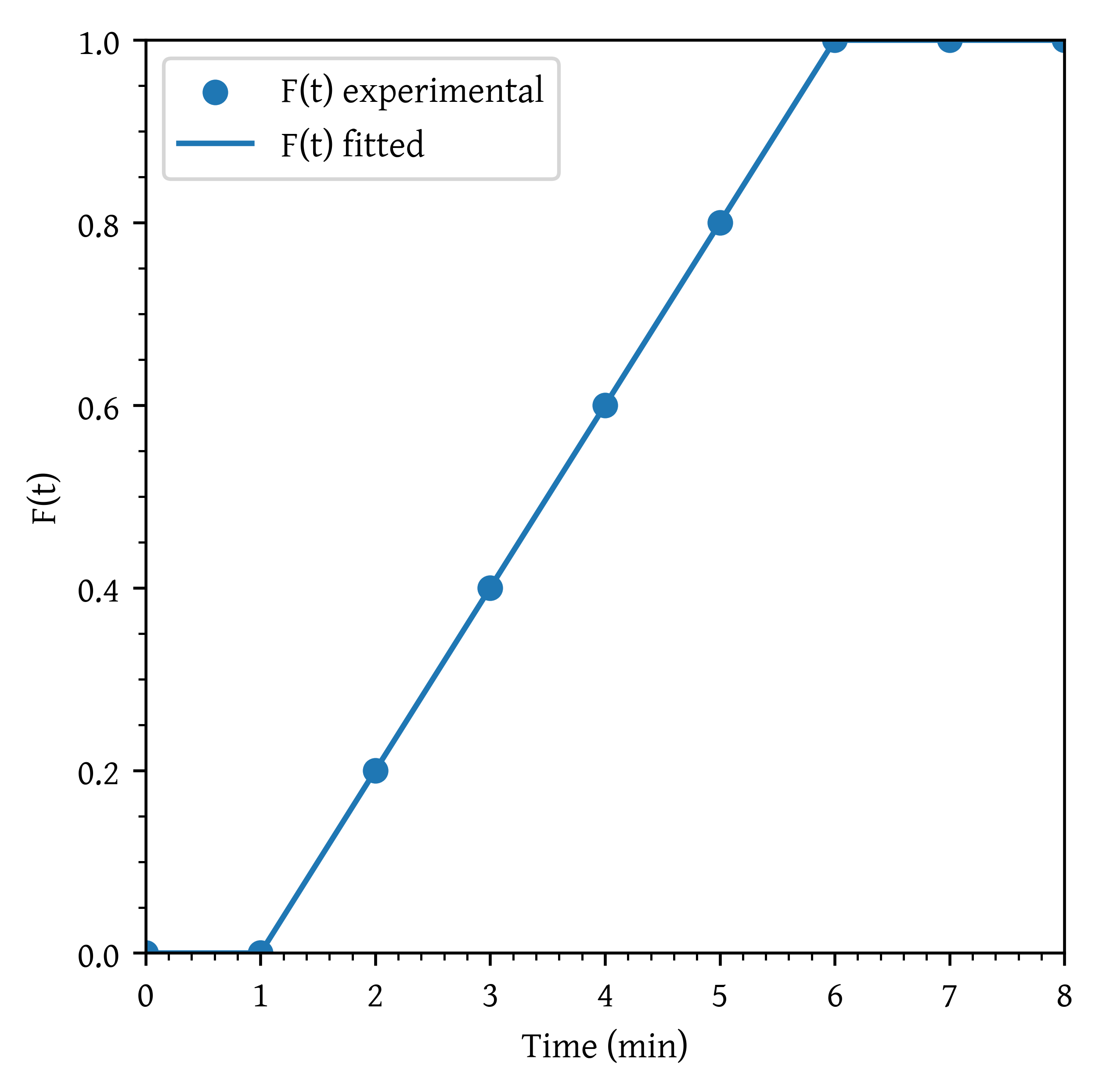

Figure 8: Cumulative distribution F(t)

To calculate E(t) as the derivative of F(t) with respect to time t, we can use the np.gradient function, which provides a numerical differentiation method. Once E(t) is calculated, we can plot it against time.

# Calculate E(t) as the derivative of F(t) with respect to t

et_plot = np.gradient(f_plot, t_plot)
et_interp = interp1d(t_plot, et_plot, kind="linear", fill_value="extrapolate")

# Plot C(t)
plt.plot(t_plot, et_plot, label='E(t)')
plt.xlabel('Time (min)')
plt.ylabel('E(t)')
plt.xlim(np.min(t_plot), np.max(t_plot))
plt.legend()
plt.show()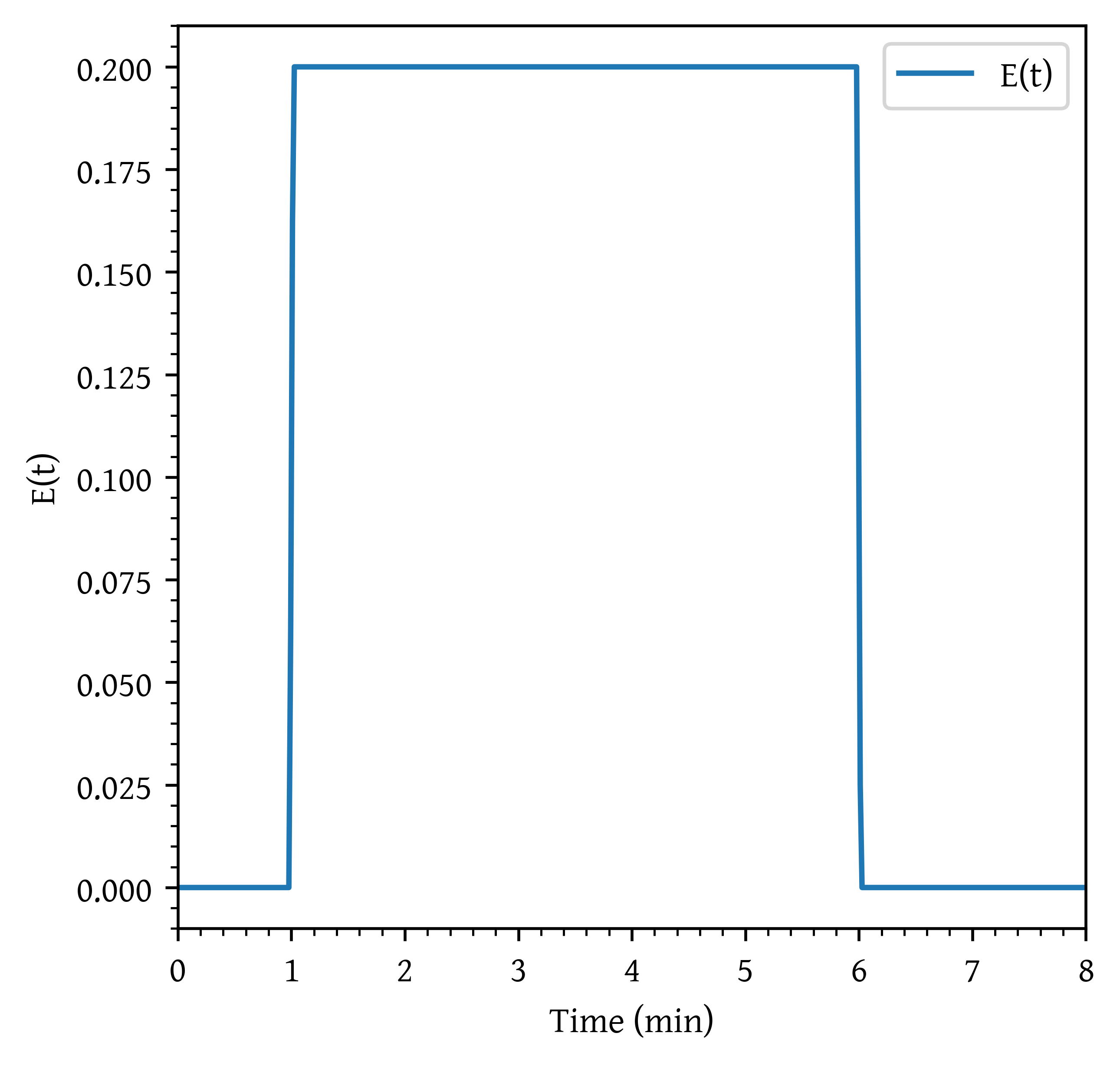

Figure 9: E Curve

Mean conversion using segragation model

Using the pulse input response in Table 1, calculate the mean conversion in the reactor for first order reaction: \ce{A ->[k] Products} with k = 0.1 [min]^{-1}.

Solution

For the first order reaction, conversion in each globule can be written as

X(t) = 1 - e^{-kt} = 1 - e^{-0.1 t}

The mean conversion can be calculated as

\bar{X} = \int_0^\infty \left( 1 - e^{-0.1 t}\right ) E(t)dt

# For data in table 1
t = data_p1["t(min)"]
c = data_p1["$C_{tracer} \\ (g/dm^3)$"]

k = 0.1
# For data in table 2
# t = data_p2["t(min)"]
# c = data_p2["C ($g/m^3$)"]

x = 1 - np.exp(-k * t)

integral_c = np.trapz(c, t)
et = c / integral_c

xet = x * et

xet_interp = PchipInterpolator(t, xet, extrapolate=True)

mean_x,_ = quad(xet_interp, 0, np.max(t))

The mean conversion is 74.8 %