In class activity: Non-isothermal reactor design

Lecture notes for chemical reaction engineering

Heat of reaction

Calculate the heat of reaction for the synthesis of ammonia from hydrogen and nitrogen at 150 °C in kcal/mol of N₂ reacted and also in kJ/mol of H₂ reacted.

$$\ce{N2 + 3H2 -> 2NH3}$$

The enthalpy of formation of ammonia at 25 °C is $H_{NH_3}^\circ (T_R) = -11020 \ cal/(mol\ \ce{NH3})$

Solution

The enthalpy of formations at 25 °C

$H_{NH_3}^\circ (T_R) = -11020 \ cal/(mol\ \ce{NH3})$

$H_{N_2}^\circ (T_R) = 0 \ cal/(mol\ \ce{NH3})$

$H_{H_2}^\circ (T_R) = 0 \ cal/(mol\ \ce{NH3})$

Heats of formation of pure components are 0.

$$\Delta H_{Rx}^\circ(T_R) = \sum_{i=1}^{N} \nu_i H_i^\circ (T_R)$$

$$\Delta H_{Rx}(T) = \Delta H_{Rx}^\circ(T_R) + \Delta C_{P}(T - T_R)$$

Getting the $C_{P}$ values from Perry’s handbook (Green and Southard (2019))

$C_{P_{H_2}}$ = 6.992 $cal/mol\ H_2\ K$; $C_{P_{N_2}}$ = 6.984 $cal/mol\ N_2\ K$; $C_{P_{NH_3}}$ = 8.92 $cal/mol\ NH_3\ K$

T = 150 + 273.15
TR = 25 + 273.15

hf_nh3 = -11020
hf_n2 = 0
hf_h2 = 0

# N2 + 3H2 -> 2 NH3
nu_n2 = -1
nu_h2 = -3
nu_nh3 = 2

# Getting the Cp values from Perry's handbook (@green2019)
cp_h2 = 6.992 # cal/mol H2 K
cp_n2 = 6.984 # cal/mol N2 K
cp_nh3 = 8.92 # cal/mol NH3 K

delta_h_tr = (nu_nh3 * hf_nh3) + (nu_n2 * hf_n2 + nu_h2 * hf_h2)
delta_cp = (nu_nh3 * cp_nh3) + (nu_n2 * cp_n2 + nu_h2 * cp_h2)

delta_h = delta_h_tr + delta_cp * (T - TR)

cal = 4.184 # J
delta_h_kj = cal * delta_h_tr + delta_cp * (T - TR)

$\Delta H_{Rx}^\circ(T_R)$ = -22.04 $kcal/mol\ N_2\ reacted$

$\Delta H_{Rx}(T)$ at 423.15 K = -93.48 $kJ/mol\ N_2\ reacted$

$$\Delta H_{Rx}(T)|_{H_2} = \frac{\nu_{N_2}}{\nu_{H_2}} \Delta H_{Rx}(T)|_{N_2}$$

$\Delta H_{Rx}(T)$ at 423.15 K = -31.16 $kJ/mol\ H_2\ reacted$

Adiabatic Liquid-Phase Isomerization of Normal Butane

Normal butane, $C_4H_{10}$, is to be isomerized to isobutane in a plug-flow reactor. Isobutane is a valuable product that is used in the manufacture of gasoline additives. For example, isooctane can be further reacted to form iso-octane. The 2014 selling price of n-butane was $1.5/gal, while the trading price of isobutane was $1.75/gal.

This elementary reversible reaction is to be carried out adiabatically in the liquid phase under high pressure using essentially trace amounts of a liquid catalyst that gives a specific reaction rate of $31.1 \, \text{h}^{-1}$ at $360 \, K$. The feed enters at $330 \, K$.

1. Calculate the PFR volume necessary to process $100,000 \, \text{gal/day}$ ($163 \, \text{kmol/h}$) at $70\%$ conversion of a mixture $90 \, \text{mol \%} \, n$-butane and $10 \, \text{mol \%} \, i$-pentane, which is considered an inert.

2. Plot and analyze $X$, $X_e$, $T_r$, and $-r_A$ down the length of the reactor.

3. Calculate the CSTR volume for $40\%$ conversion.

Additional information:

$\Delta H^{\circ}_{Rx} = -6900 \, \text{J/mol} \, n$-butane,

Activation energy = $65.7 \, \text{kJ/mol}$

$K_c = 3.03$ at $60°C$,

$C_{A0} = 9.3 \, \text{mol/dm}^3 = 9.3 \, \text{kmol/m}^3$

Butane: $C_{P_{n-B}} = 141 \, J/mol \cdot K$; $C_{P_{i-B}} = 141 \, J/mol \cdot K$

i-Pentane: $C_{P_{i-P}} = 161 \, J/mol \cdot K$

Solution

PFR algorithm

1. Mole balance

$$F_{A0} \frac{dX}{dV} = -r_A \tag{1}$$

2. Rate law

$$-r_A = k \left( C_A - \frac{C_B}{K_C}\right) \tag{2}$$

$$k = k(T_1) \exp \left[ \frac{E}{R} \left( \frac{1}{T_1} - \frac{1}{T}\right)\right] \tag{3}$$

$$K_C = K_C(T_2) \exp \left[ \frac{\Delta H_{Rx}}{R} \left( \frac{1}{T_2} - \frac{1}{T}\right)\right] \tag{4}$$

3. Stoichiometry

$$C_A = C_{A0} (1 - X) \tag{5}$$

$$C_B = C_{A0} X \tag{6}$$

4. Energy balance

$$\dot Q - \dot W_s - F_{A0} \sum_{i=1}^{N} \Theta_i C_{P_i} \left[ T_{i} - T_{i0}\right] - \Delta H_{Rx} F_{A0} X = 0 \tag{7}$$

From problem statement:

Adiabatic: $\dot Q$ = 0

No work: $\dot W_s$ = 0

$\Delta C_{P} = C_{P_A} - C_{P_B}$ = 141 - 141 = 0

Substituting in Equation 7

$$T = T_0 + \frac{ \left( -\Delta H^\circ_{Rx} \right) X_{EB}}{\sum \Theta_i C_{Pi}} \tag{8}$$

5. Solve

Solve equations 1 to 7 simultaneously.

import numpy as np
import matplotlib.pyplot as plt
from scipy.integrate import solve_ivp

# Constants
K0 = 31.1 # 1/h
T_K0 = 360 # K

KC0 = 3.3
T_KC0 = 60 + 273.15 # K

E = 65700 # J/mol 
R = 8.314 # J/mol K

DELTAHR = -6900 # J/mol

def adiabatic_pfr( V, y, *args ):

  X = y[0]
  (fa0,ca0, T0, theta, cp) = args

  sum_cp =  np.sum(theta * cp)

  T = T0 + (-DELTAHR) * X / sum_cp

  k = K0 * np.exp((E/R) * (1/T_K0 - 1/T))
  Kc = KC0 * np.exp((DELTAHR/R) * (1/T_KC0 - 1/T))

  ca = ca0 * ( 1 - X )
  cb = ca0 * X

  rate = k * (ca - cb/Kc)

  dXdV = rate/fa0

  return dXdV

# Problem data
ya0 = 0.9
yi0 = 0.1
fa = 163.0 # kmol/h
fa0 = ya0 * fa 
ca0 = 9.3   # kmol/m3

T0 = 330 # K

# n-butane = comp 1; i-butane = comp 2; i-Pentane = component 3

theta = np.array([1, 0, yi0/ya0])
cp = np.array([141, 141, 161])
                 
# Initial condition
y0 = [0]
args = (fa0, ca0, T0, theta, cp)
v_final = 5
sol = solve_ivp(adiabatic_pfr, [0, v_final], y0, args=args, dense_output=True)

v = np.linspace(0,v_final, 1000)
x = sol.sol(v)[0]

pfr_07 = v[np.argmax(x > 0.7)]

PFR volume required to obtain a conversion of 0.7 = 2.24 $m^3$.

# recalculate other quantities for plotting
sum_cp =  np.sum(theta * cp)
T = T0 + (-DELTAHR) * x / sum_cp
Kc = KC0 * np.exp((DELTAHR/R) * (1/T_KC0 - 1/T))
xe = Kc/(1 + Kc)

Temperature profile

plt.plot(v,T, label='Temperature')

plt.xlabel('Volume ($m^3$)')
plt.ylabel('Temperature (K)')

plt.xlim(0,v_final)
plt.ylim(T0,)

plt.show()

Figure 1

Conversion profile

plt.plot(v,x, label='$X$')
plt.plot(v,xe, label='$X_e$')

plt.xlabel('Volume ($m^3$)')
plt.ylabel('Conversion')

plt.xlim(0,v_final)
plt.ylim(0,1)

plt.legend()
plt.show()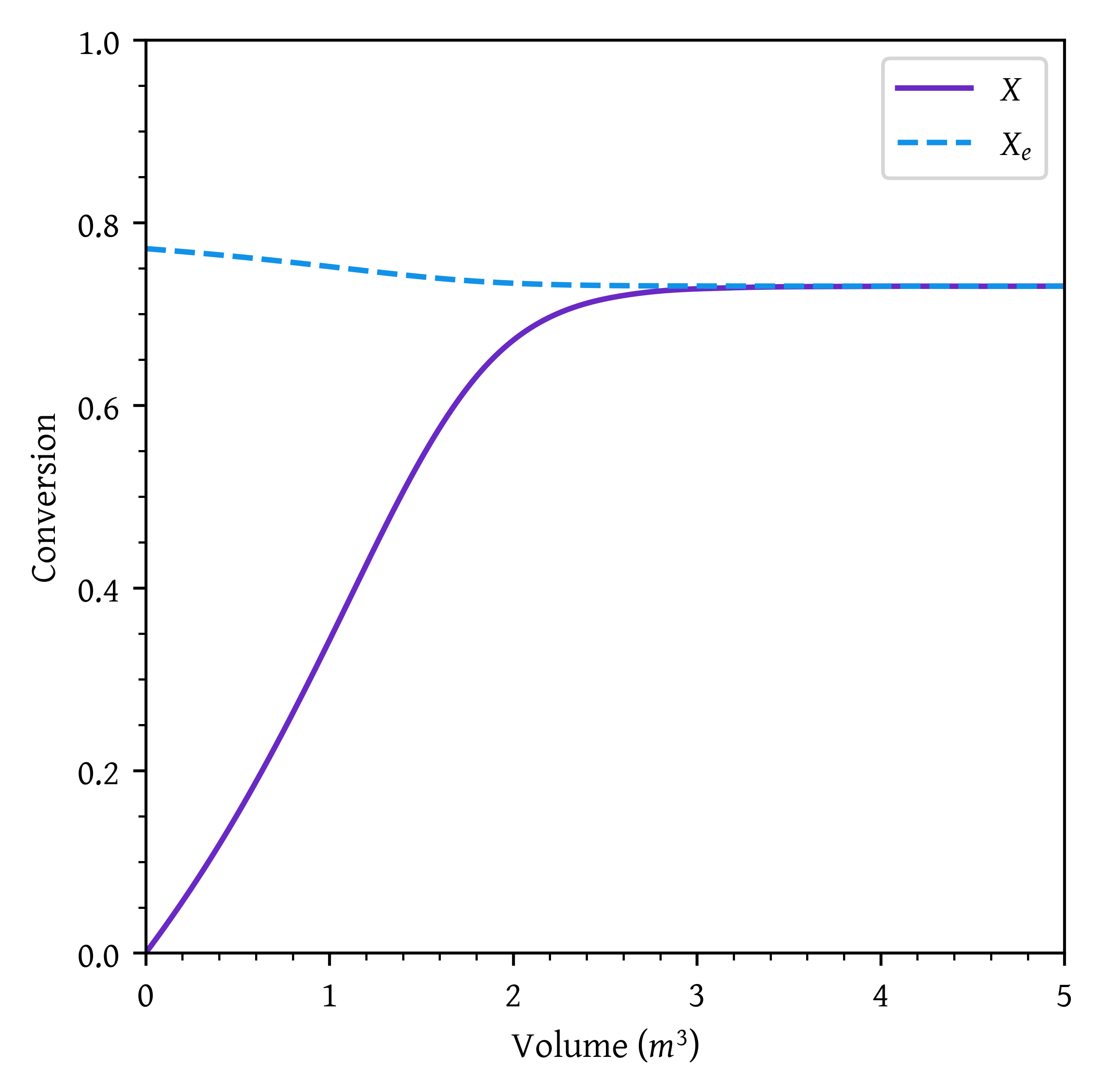

Figure 2: Conversion profile

CSTR volume

pfr_04 = v[np.argmax(x > 0.4)]

temp_04 = T[np.argmax(x > 0.4)]
kc_04 = Kc[np.argmax(x > 0.4)]
k_04 = K0 * np.exp((E/R) * (1/T_K0 - 1/temp_04))

ca = ca0 * ( 1 - 0.4 )
cb = ca0 * 0.4
rate = k_04 * (ca - cb/kc_04)

cstr_04 = fa0 * 0.4/ rate

PFR volume required to obtain a conversion of 0.4 = 1.14 $m^3$.

CSTR volume required to obtain a conversion of 0.4 = 0.97 $m^3$.

Adiabatic Equilibrium Temperature

For the elementary liquid-phase reaction

$\ce{A <=> B}$

Make a plot of equilibrium conversion as a function of temperature.

1. Combine the rate law and stoichiometric table to write $-r_A$ as a function of $k$, $C_{A0}$, $X$, and $X_e$.

2. Determine the adiabatic equilibrium temperature and conversion when pure A is fed to the reactor at a temperature of 300 K.

3. What is the CSTR volume to achieve 90% of the adiabatic equilibrium conversion for $\dot{v}_0 = 5 \, \text{dm}^3/\text{min}$?

Additional information:†

$H_A^\circ(298 \, K) = -40,000 \, \text{cal/mol}$

$H_B^\circ(298 \, K) = -60,000 \, \text{cal/mol}$

$C_{P,A} = 50 \, cal/mol \cdot K$

$C_{P,B} = 50 \, cal/mol \cdot K$

$K_c = 100,000$ at 298 K, $k = 10^{-3} \exp \left( \frac{E}{R} \left( \frac{1}{298} - \frac{1}{T} \right) \right) \text{min}^{-1}$ with $E = 10,000 \, \text{cal/mol}$

Solution

1. Rate law

$$-r_A = k \left( C_A - \frac{C_B}{K_C}\right) \tag{9}$$

$$k = k(T_1) \exp \left[ \frac{E}{R} \left( \frac{1}{T_1} - \frac{1}{T}\right)\right] \tag{10}$$

$$K_C = K_C(T_2) \exp \left[ \frac{\Delta H_{Rx}}{R} \left( \frac{1}{T_2} - \frac{1}{T}\right)\right] \tag{11}$$

2. Equilibrium

$$K_e = \frac{C_{Be}}{C_{Ae}} \tag{12}$$

3. Stoichiometry

$$C_A = C_{A0} (1 - X) \tag{13}$$

$$C_B = C_{A0} X \tag{14}$$

Combining Equation 9, Equation 12, Equation 13, and Equation 14

$$X_e = \frac{K_e(T)}{1 + K_e(T)} \tag{15}$$

4. Energy balance

$$\dot Q - \dot W_s - F_{A0} \sum_{i=1}^{N} \Theta_i C_{P_i} \left[ T_{i} - T_{i0}\right] - \Delta H_{Rx} F_{A0} X = 0 \tag{16}$$

From problem statement:

Adiabatic: $\dot Q$ = 0

No work: $\dot W_s$ = 0

$\Delta C_{P} = C_{P_A} - C_{P_B}$ = 141 - 141 = 0

Substituting in Equation 16

$$X_{EB} = \frac { \sum \Theta_i C_{P_i} \left[ T_{i} - T_{0}\right] } {- \Delta H_{Rx}^\circ (T_R) } \tag{17}$$

import numpy as np
import matplotlib.pyplot as plt
from scipy.integrate import solve_ivp
from scipy.optimize import fsolve

# Constants
HF_A = -40000 # cal/mol
HF_B = -60000 # cal/mol

CP_A = 50 # cal/mol K
CP_B = 50 # cal/mol K

# A <-> B
D_CP = CP_B - CP_A

KE0 = 100000
T_KE0 = 298 # K

K0 = 1e-3 # 1/h
T_K0 = 298 # K

E = 10000  # cal/mol
R = 1.987 # cal/mol K

DELTAHR = HF_B - HF_A

T0 = 300 # K

Ke = lambda T: KE0 * np.exp((DELTAHR/R) * (1/T_KE0 - 1/T))
Xe = lambda T: Ke(T)/(1 + Ke(T))
Xeb = lambda T, T0: CP_A * (T - T0)/(-DELTAHR)

intersect = lambda T: Xe(T) - Xeb(T, T0)

sol = fsolve(intersect, T0)

T_adiab = sol[0]
X_eadiab = Xe( T_adiab )

Adiabatic equilibrium temperature = 460.40 K.

Adiabatic equilibrium conversion = 0.40.

T_final = T0 + 300
temperatures = np.linspace(T0, T_final , 100)
conv_eb = Xeb(temperatures, T0)
conv_eq = Xe(temperatures)

plt.plot(temperatures,conv_eb, label="$X_{eb}$")
plt.plot(temperatures,conv_eq, label="$X_{eq}$")

plt.xlabel('Temperature (K)')
plt.ylabel('Conversion')

plt.xlim(T0, T_final)
plt.ylim(0,1)
plt.legend()
plt.show()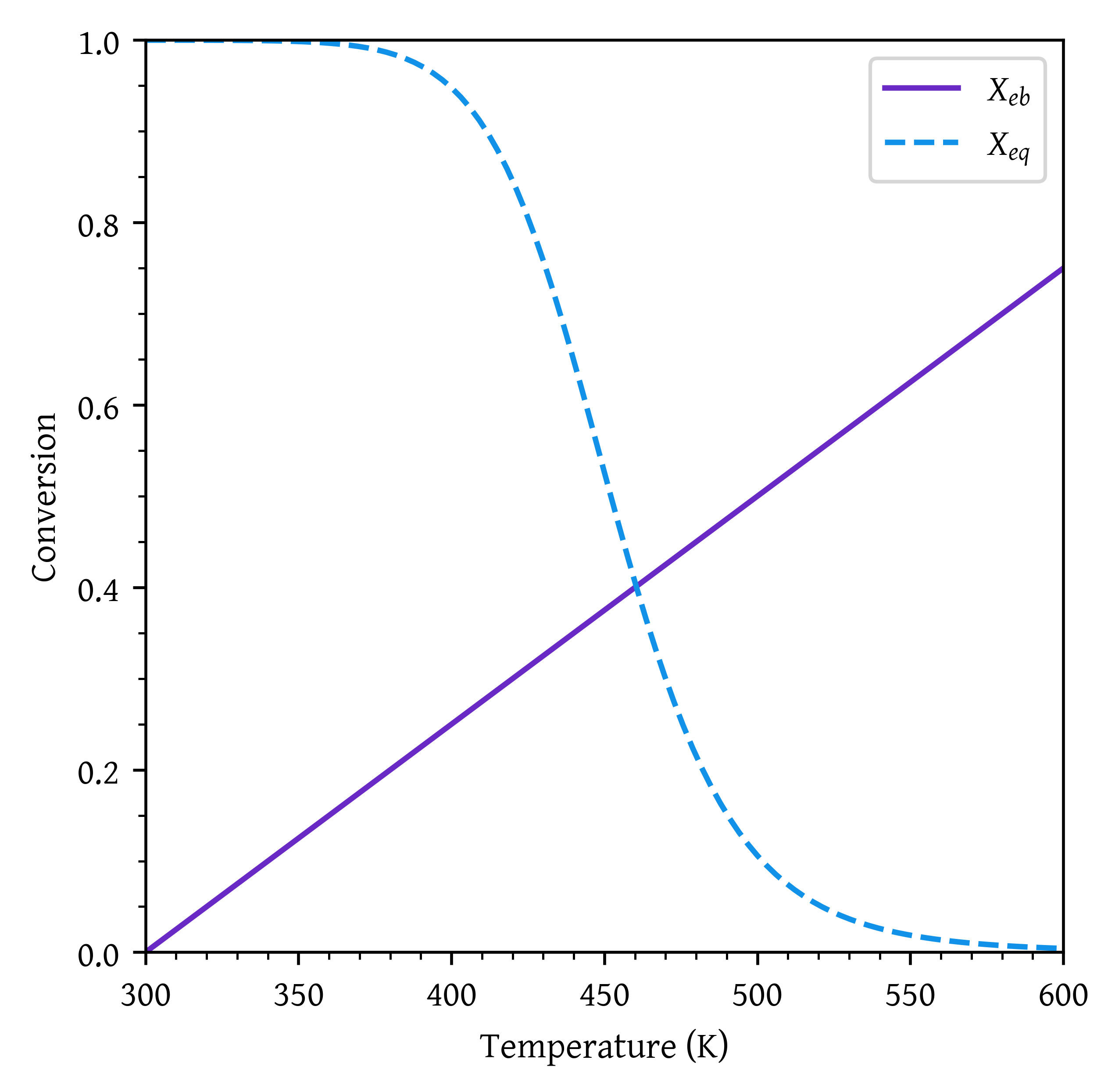

Figure 3: Conversion vs. temperatures

CSTR Volume

$$V = \frac{F_{A0} X}{ -r_A } \tag{18}$$

Calculate temperature corresponding to X = 0.9 X_e

$$T = T_0 + \frac{ \left( -\Delta H^\circ_{Rx} \right) X_{EB}}{\sum \Theta_i C_{Pi}} \tag{19}$$

Calculate rate at this temperature using Equation 9 and Equation 10.

k = lambda T: K0 * np.exp((E/R) * (1/T_K0 - 1/T))

v_0 = 5 # dm^3/min
x_cstr = 0.9 * X_eadiab

def v_cstr(x, xin, t0, ca0, v_0):
  t_cstr = t0 + (x - xin)*(-DELTAHR)/CP_A
  rate = k(t_cstr) * ca0 * (1 - (x/Xe(t_cstr)))
  v_cstr = v_0 * ca0 * x/rate
  return v_cstr,t_cstr

V_cstr,T_cstr = v_cstr(x_cstr,0,T0,1.0,v_0)

For a CSTR to achieve a conversion of 90% of $X_e$ (= 0.36), volume required is 17.57 $dm^3$. The CSTR operates at 444.36 $K$.

Interstage Cooling for Highly Exothermic Reactions

What conversion could be achieved in the previous example if two interstage coolers that had the capacity to cool the exit stream to 350 K were available? Also, determine the heat duty of each exchanger for a molar feed rate of A of 40 mol/s. Assume that 95% of the equilibrium conversion is achieved in each reactor. The feed temperature to the first reactor is 300 K.

Solution

# Stage 1

fa0 = 40.0 # mol/s

x1 = 0.95 * X_eadiab
v_cstr1, t_cstr1 = v_cstr(x1,0,T0,1.0,v_0)

Stage 1: $X_{1}$ = 0.38. $V_{CSTR}$ = 25.69 $dm^3$. $T_{CSTR}$ = 452.38 $K$.

Heat Load:

$$\dot Q - \dot W_s - \sum F_{i} C_{P_i}(T_2 - T_1) = 0 \tag{20}$$

$\dot W_s = 0$; $C_{P_A} = C_{P_B}$

$$\dot Q = (F_{A} + F_B) C_{P_A}(T_2 - T_1) \tag{21}$$

T_ic = 350
qdot1 = fa0 * CP_A * (T_ic - t_cstr1)

Stage 1 cooling requirement : $\dot Q_1$ = -204.76 $kcal/s$.

# Stage 2
# find adiabatic conversion and temperature for second stage

intersect = lambda T: Xe(T) - ( x1 + Xeb(T, T_ic))

sol = fsolve(intersect, T0)

T2_adiab = sol[0]
X2_eadiab = Xe( T2_adiab )

x2 = X2_eadiab * 0.95

v_cstr2, t_cstr2 = v_cstr(x2,x1,T_ic,1.0,v_0)
qdot2 = fa0 * CP_A * (T_ic - t_cstr2)

Stage 2: $X_{2}$ = 0.58. $T_{adiab,2}$ = 442.93 $K$. $V_{CSTR,2}$ = 71.24 $dm^3$. $T_{CSTR,2}$ = 430.66 $K$.

Stage 2 cooling requirement : $\dot Q_2$ = -161.33 $kcal/s$.

# Stage 3
# find adiabatic conversion and temperature for second stage

intersect = lambda T: Xe(T) - ( x2 + Xeb(T, T_ic))

sol = fsolve(intersect, T0)

T3_adiab = sol[0]
X3_eadiab = Xe( T3_adiab )

x3 = X3_eadiab * 0.95

v_cstr3, t_cstr3 = v_cstr(x3,x2,T_ic,1.0,v_0)
qdot3 = fa0 * CP_A * (T_ic - t_cstr3)

Stage 3: $X_{3}$ = 0.74. $T_{adiab,3}$ = 428.03 $K$. $V_{CSTR,3}$ = 195.40 $dm^3$. $T_{CSTR,3}$ = 412.47 $K$.

Stage 3 cooling requirement : $\dot Q_3$ = -124.95 $kcal/s$.

Production of Acetic Anhydride

Jeffreys, in a treatment of the design of an acetic anhydride manufacturing facility, states that one of the key steps is the endothermic vapor-phase cracking of acetone to ketene and methane.

The reaction is as follows: $$\ce{ CH3COCH3 -> CH2CO + CH4}$$

He states further that this reaction is first-order with respect to acetone and that the specific reaction rate can be expressed by

$$\ln k = 34.34 - \frac{34,222}{T}$$

where $k$ is in reciprocal seconds and $T$ is in Kelvin. In this design it is desired to feed 7850 kg of acetone per hour to a tubular reactor. The reactor consists of a bank of 1000 one-inch schedule 40 tubes. We shall consider four cases of heat exchanger operation. The inlet temperature and pressure are the same for all cases at 1035 K and 162 kPa (1.6 atm) and the entering heating-fluid temperature available is 1250 K.

A bank of 1000 one-inch, schedule 40 tubes 1.79 m in length corresponds to 1.0 m³ (0.001 m³/tube = 1.0 dm³/tube) and gives 20% conversion. Ketene is unstable and tends to explode, which is a good reason to keep the conversion low. However, the pipe material and schedule size should be checked to learn if they are suitable for these temperatures and pressures. The heat-exchange fluid has a flow rate, $\dot{m}_c$, of 0.111 mol/s, with a heat capacity of 34.5 J/mol·K.

The cases are as follows:

• Case 1: The reactor is operated adiabatically.
• Case 2: Constant heat-exchange fluid temperature $T_a = 1250$ K.
• Case 3: Co-current heat exchange with $T_{a0} = 1250$ K.
• Case 4: Countercurrent heat exchange with $T_{a0} = 1250$ K.

Additional information:

• For acetone (A): $\Delta H^{\circ}_{A}(T_R) = -216.67$ kJ/mol, $C_{p,A} = 163$ J/mol·K
• For ketene (B): $\Delta H^{\circ}_{B}(T_R) = -61.09$ kJ/mol, $C_{p,B} = 83$ J/mol·K
• For methane (C): $\Delta H^{\circ}_{C}(T_R) = -74.81$ kJ/mol, $C_{p,C} = 71$ J/mol·K

The overall heat transfer coefficient $Ua = 110$ $J/s \cdot m^3 \cdot K$.

Solution

Reaction: $\ce {A -> B + C}$

1. Mole balance

$$\frac{dX}{dV} = -\frac{r_A}{F_{A0}}$$

2. Rate law

$$-r_A = k C_A$$

3. Stoichiometry $$C_A = \frac{ C_{A0} (1 - X) }{ (1 + \epsilon X) } \frac{ T_0 }{ T }$$

4. Energy balance

Reactor balance

$$\frac{dT}{dV} = \frac{ U a (T_a - T) + r_A \left[ \Delta H_{Rx}^\circ+ \Delta C_P (T - T_R)\right] }{ F_{A0} \left( \sum \Theta_i C_{P_i} + X \Delta C_P \right) }$$

Heat exchanger

$$\frac{dT_a}{dV} = \frac{ U a (T - T_a) }{ \dot m_C C_{P_C} }$$

import numpy as np
import matplotlib.pyplot as plt
from scipy.integrate import solve_ivp

# Constants
R = 8.314 # J/mol K
TR = 298 # K
# Components: 1: A(acetone), 2: B(ketene), 3: C(methane)
HF = np.array ([-216.67, -61.09, -74.81])*1000   # J/mol
CP = np.array ([163.0, 83.0, 71.0]) # J/mol K
MW = np.array ([58.0, 42.0, 20.0]) # g/mol

k = lambda t: np.exp( 34.34 - 34222/t )
# k = lambda t: 3.58 * np.exp( 34222 * (1/1035 - 1/t))

def pfr (v, x, *args):
  X, T, Ta = x
  (fa0, ca0, T0, epsilon, delta_hr_tr, delta_cp, theta, UA, mc, cpc) = args

  ca = ca0 * (( 1 - X ) / ( 1 + epsilon * X )) * (T0/T)
  rate = k(T) * ca # -r_A
  delta_h = delta_hr_tr + delta_cp * (T - TR)

  dxdv = rate/fa0
  dtdv = (UA * ( Ta - T ) + (-rate * delta_h))/( fa0 * ( np.sum(theta * CP) + X * delta_cp) )
  dtadv = UA * ( T - Ta )/ (mc * cpc)

  return [dxdv, dtdv, dtadv]

# Data

nu = np.array ([-1.0, 1.0, 1.0]) # stoichiometric coefficients

f0 = 7850 # kg/h
T0 = 1035.0 # K
P0 = 162.0e3 # Pa

n_tubes = 1000
d_tube = 26.64e-3  # 1" schedule 40 pipe inner diameter mm
Ta0 = 1250 # K
a = 4/d_tube
U = 110.0 # J/s m^3 K
UA = U * a


mc = 0.111 # mol/s
cpc = 34.5 # J/mol K

# inlet mole fraction
y0 = np.array ([1.0, 0.0, 0.0])
theta = np.array([1.0, 0.0, 0.0])

fa0 = (f0 / ( y0[0] * MW[0])) / n_tubes # kmol/h
fa0 = fa0 * (1000/3600)  # mol/s

pa0 = y0[0] * P0
ca0 = pa0/(R * T0)
v_0 = fa0/ca0
ya0 = y0[0]

# Heat of reaction at 298K
delta_hr_tr = np.sum(HF * nu)
delta_cp = np.sum(CP * nu)

epsilon = ya0 * np.sum(nu)

	Parameter values
$\Delta H^\circ_{Rx} (T_R)$ = 80770.00 $J/mol$	$\Delta C_P$ = -9.00 $J/mol\ K$	$T_0$ = 1035.00 K
$F_{A0}$ = 3.76e-02 mol/s	$C_{A0}$ = 18.83 $mol/m^3$	$T_R$ = 298.00 K
$C_{P_A}$ = 163.00 $J/mol\ K$	$Ua$ = 16516.52 $J/m^3\ s\ K$	$\dot m_C$ = 0.11 $mol/s$
$C_{P_C}$ = 34.50 $J/mol\ K$		$V_f$ = 0.001 $m^3$

args = (fa0, ca0, T0, epsilon, delta_hr_tr, delta_cp, theta, 0, mc, cpc)

initial_conditions = np.array([0, T0, Ta0])
v_final = 0.005

sol = solve_ivp(pfr, [0, v_final], initial_conditions, args=args, dense_output=True)
v = np.linspace(0,v_final, 1000)
x = sol.sol(v)[0]
T = sol.sol(v)[1]
Ta = sol.sol(v)[2]

fig, ax1 = plt.subplots()

# Plot x on the original y-axis
plt_x = ax1.plot(v, x, color='#105e5d', label='X')
ax1.set_xlabel('volume ($m^3$)')
ax1.set_ylabel('Conversion')
ax1.set_xlim(0,v[-1])
ax1.set_ylim(0,)

# Create a second y-axis for T and Ta
ax2 = ax1.twinx()
plt_t = ax2.plot(v, T, label='T') 
# plt_ta = ax2.plot(v, Ta, label='Ta') 
ax2.set_ylabel('Temperature (K)')

ax2.set_xlim(0,v[-1])
ax2.set_ylim(top=T0)

arrow_properties = dict(arrowstyle="<-,head_length=0.7,head_width=0.25",
                        color="black")

ax1.annotate('', xy=(v[100],x[100]), xytext=(v[0], x[100]),arrowprops=dict(arrowstyle="<-"))
ax2.annotate('', xy=(v[100],T[100]), xytext=(v[200], T[100]),arrowprops=dict(arrowstyle="<-"))

# fig.tight_layout()
handles, labels = [], []
for ax in [ax1, ax2]:
    for handle, label in zip(*ax.get_legend_handles_labels()):
        handles.append(handle)
        labels.append(label)
plt.legend(handles, labels)
plt.show()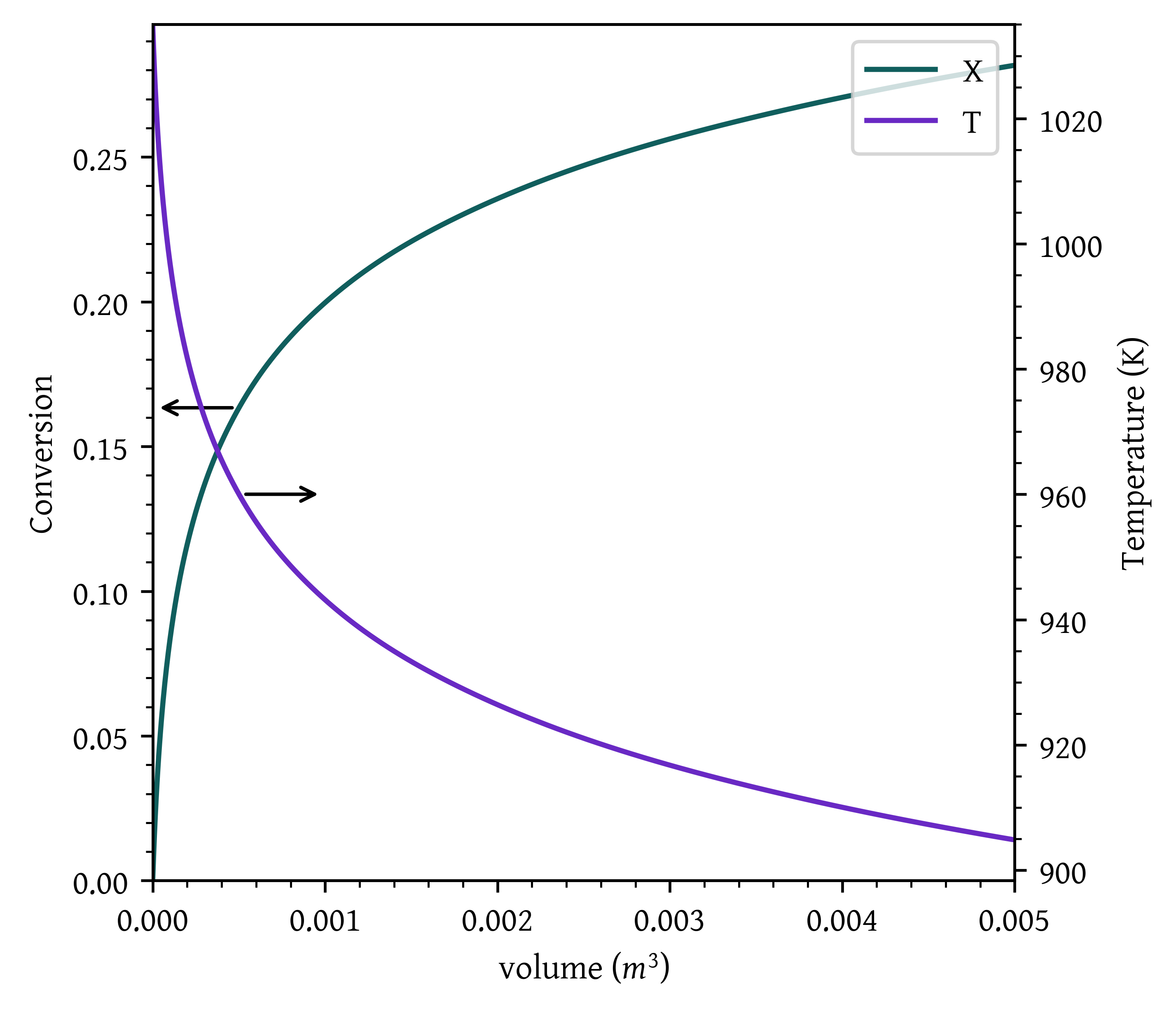

Adiabatic conversion and temperature

def pfr_const_heatex_fluid_T (v, x, *args):
  X, T, Ta = x
  (fa0, ca0, T0, epsilon, delta_hr_tr, delta_cp, theta, UA, mc, cpc) = args

  ca = ca0 * (( 1 - X ) / ( 1 + epsilon * X )) * (T0/T)
  rate = k(T) * ca # -r_A
  delta_h = delta_hr_tr + delta_cp * (T - TR)

  dxdv = rate/fa0
  dtdv = (UA * ( Ta - T ) + (-rate * delta_h))/( fa0 * ( np.sum(theta * CP) + X * delta_cp) )
  dtadv = 0.0

  return [dxdv, dtdv, dtadv]


args = (fa0, ca0, T0, epsilon, delta_hr_tr, delta_cp, theta, UA, mc, cpc)

initial_conditions = np.array([0, T0, Ta0])
v_final = 0.001

sol = solve_ivp(pfr_const_heatex_fluid_T, [0, v_final], initial_conditions, args=args, dense_output=True)
v = np.linspace(0,v_final, 1000)
x = sol.sol(v)[0]
T = sol.sol(v)[1]
Ta = sol.sol(v)[2]

fig, ax1 = plt.subplots()

# Plot x on the original y-axis
plt_x = ax1.plot(v, x, color='#105e5d', label='X')
ax1.set_xlabel('volume ($m^3$)')
ax1.set_ylabel('Conversion')
ax1.set_xlim(0,v[-1])
ax1.set_ylim(0,)

# Create a second y-axis for T and Ta
ax2 = ax1.twinx()
plt_t = ax2.plot(v, T, label='T') 
# plt_ta = ax2.plot(v, Ta, label='Ta') 
ax2.set_ylabel('Temperature (K)')

ax2.set_xlim(0,v[-1])

arrow_properties = dict(arrowstyle="<-,head_length=0.7,head_width=0.25",
                        color="black")

ax1.annotate('', xy=(v[100],x[100]), xytext=(v[0], x[100]),arrowprops=dict(arrowstyle="<-"))
ax2.annotate('', xy=(v[100],T[100]), xytext=(v[200], T[100]),arrowprops=dict(arrowstyle="<-"))

# fig.tight_layout()
handles, labels = [], []
for ax in [ax1, ax2]:
    for handle, label in zip(*ax.get_legend_handles_labels()):
        handles.append(handle)
        labels.append(label)
plt.legend(handles, labels)
plt.show()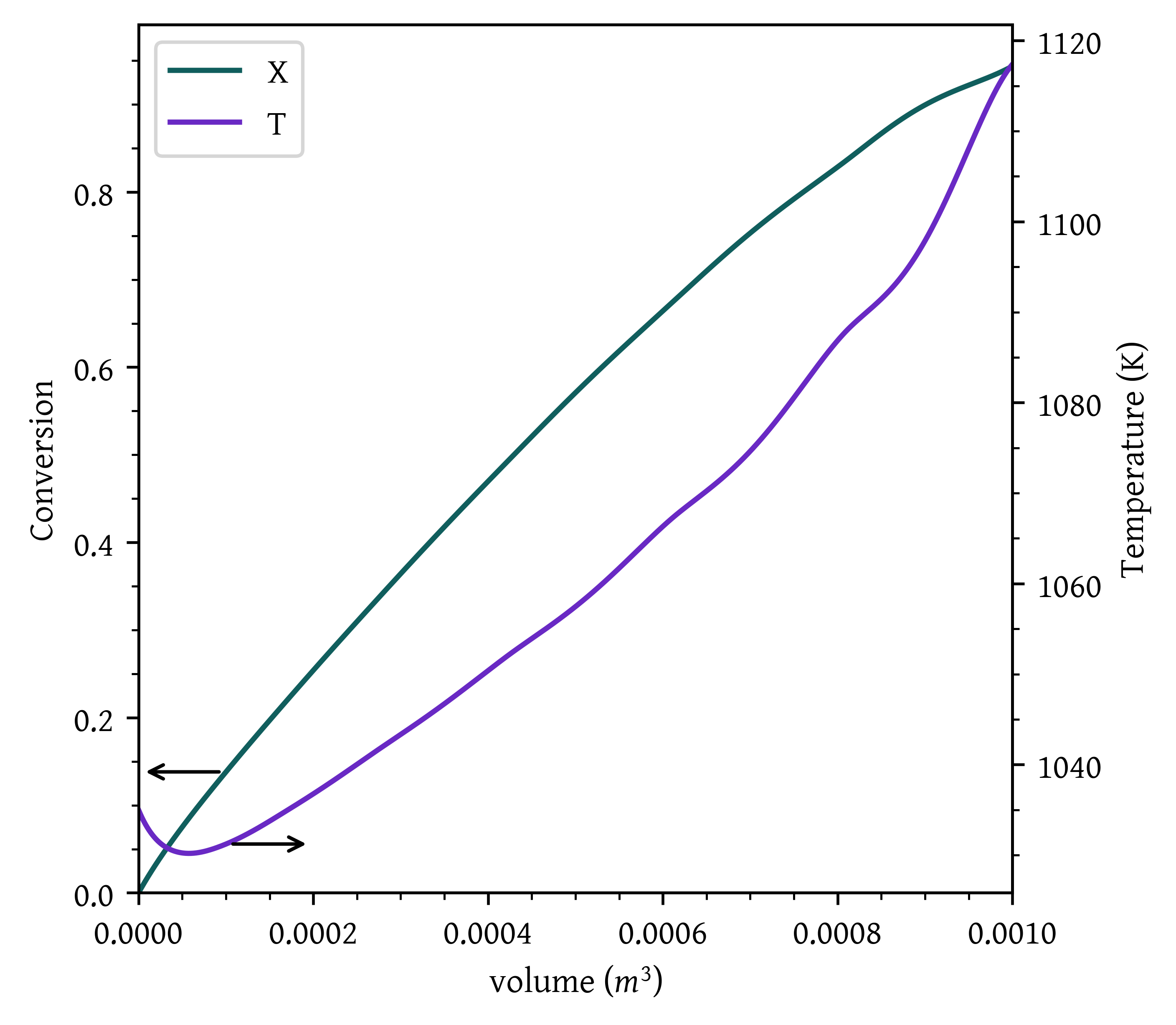

Constant heat exchange fluid temperature: conversion and temperature

args = (fa0, ca0, T0, epsilon, delta_hr_tr, delta_cp, theta, UA, mc, cpc)

initial_conditions = np.array([0, T0, Ta0])
v_final = 0.001

sol = solve_ivp(pfr, [0, v_final], initial_conditions, args=args, dense_output=True)
v = np.linspace(0,v_final, 1000)
x = sol.sol(v)[0]
T = sol.sol(v)[1]
Ta = sol.sol(v)[2]

fig, ax1 = plt.subplots()

# Plot x on the original y-axis
plt_x = ax1.plot(v, x, color='#105e5d', label='X')
ax1.set_xlabel('volume ($m^3$)')
ax1.set_ylabel('Conversion')
ax1.set_xlim(0,v[-1])
ax1.set_ylim(0,)

# Create a second y-axis for T and Ta
ax2 = ax1.twinx()
plt_t = ax2.plot(v, T, label='T') 
plt_ta = ax2.plot(v, Ta, label='Ta') 
ax2.set_ylabel('Temperature (K)')

ax2.set_xlim(0,v[-1])
ax2.set_ylim(top=Ta0)

arrow_properties = dict(arrowstyle="<-,head_length=0.7,head_width=0.25",
                        color="black")

ax1.annotate('', xy=(v[100],x[100]), xytext=(v[0], x[100]),arrowprops=dict(arrowstyle="<-"))
ax2.annotate('', xy=(v[100],T[100]), xytext=(v[200], T[100]),arrowprops=dict(arrowstyle="<-"))
ax2.annotate('', xy=(v[100],Ta[100]), xytext=(v[200], Ta[100]),arrowprops=dict(arrowstyle="<-"))

# fig.tight_layout()
handles, labels = [], []
for ax in [ax1, ax2]:
    for handle, label in zip(*ax.get_legend_handles_labels()):
        handles.append(handle)
        labels.append(label)
plt.legend(handles, labels)
plt.show()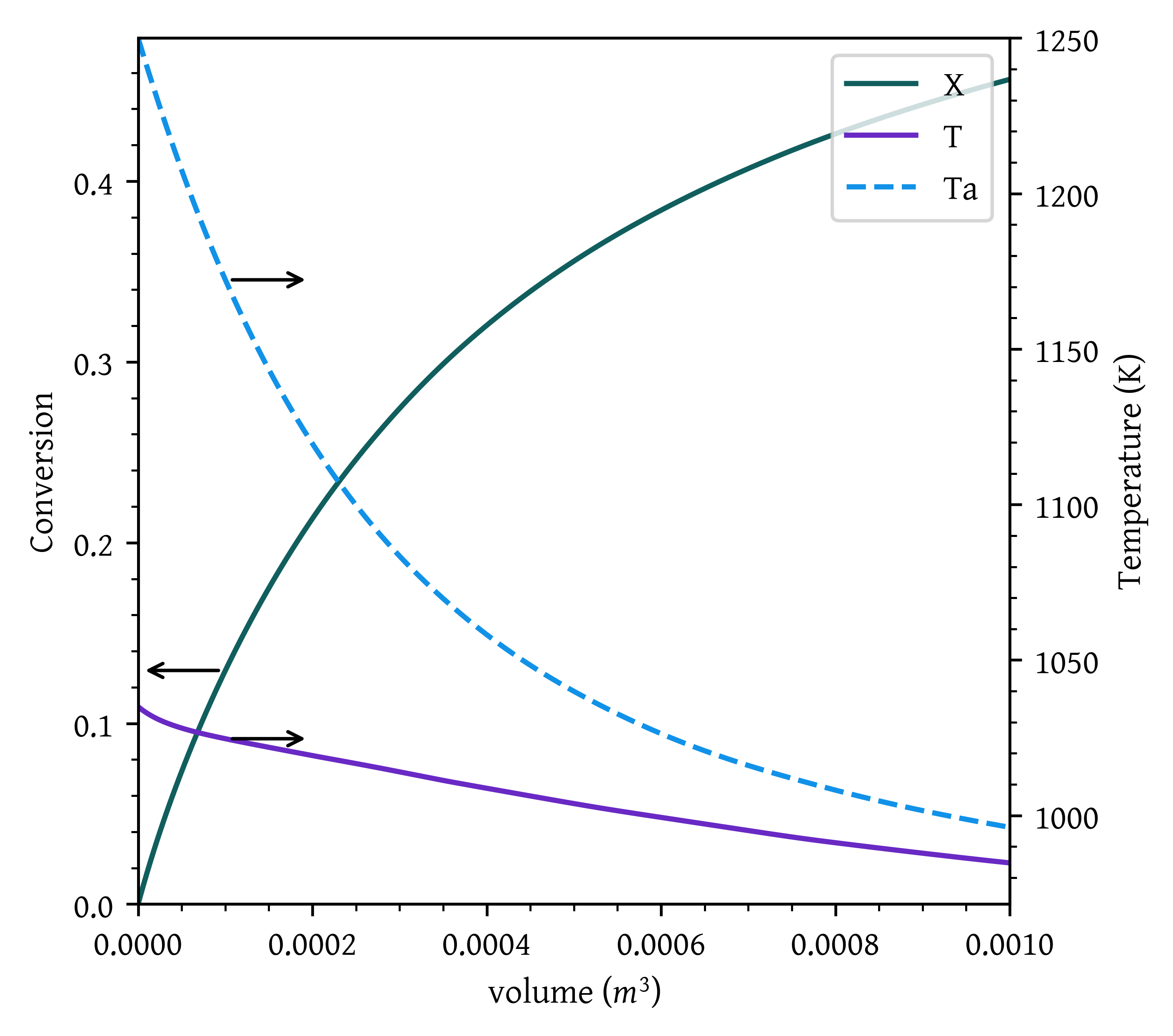

Cocurrent heat exchange: conversion and temperature

def pfr_countercurrent_exchange (v, x, *args):
  X, T, Ta = x
  (fa0, ca0, T0, epsilon, delta_hr_tr, delta_cp, theta, UA, mc, cpc) = args

  ca = ca0 * (( 1 - X ) / ( 1 + epsilon * X )) * (T0/T)
  rate = k(T) * ca # -r_A
  delta_h = delta_hr_tr + delta_cp * (T - TR)

  dxdv = rate/fa0
  dtdv = (UA * ( Ta - T ) + (-rate * delta_h))/( fa0 * ( np.sum(theta * CP) + X * delta_cp) )
  dtadv = - UA * ( T - Ta )/ (mc * cpc)

  return [dxdv, dtdv, dtadv]


v_final = 0.001

# This temperature needs to be guessed for Ta to be 1250 at V = V_final
Ta0 = 995.15

args = (fa0, ca0, T0, epsilon, delta_hr_tr, delta_cp, theta, UA, mc, cpc)

initial_conditions = np.array([0, T0, Ta0])

sol = solve_ivp(pfr_countercurrent_exchange, [0, v_final], initial_conditions, args=args, dense_output=True)
v = np.linspace(0,v_final, 1000)
x = sol.sol(v)[0]
T = sol.sol(v)[1]
Ta = sol.sol(v)[2]

fig, ax1 = plt.subplots()

# Plot x on the original y-axis
plt_x = ax1.plot(v, x, color='#105e5d', label='X')
ax1.set_xlabel('volume ($m^3$)')
ax1.set_ylabel('Conversion')
ax1.set_xlim(0,v[-1])
ax1.set_ylim(0,)

# Create a second y-axis for T and Ta
ax2 = ax1.twinx()
plt_t = ax2.plot(v, T, label='T') 
plt_ta = ax2.plot(v, Ta, label='Ta') 
ax2.set_ylabel('Temperature (K)')

ax2.set_xlim(0,v[-1])

arrow_properties = dict(arrowstyle="<-,head_length=0.7,head_width=0.25",
                        color="black")

ax1.annotate('', xy=(v[200],x[200]), xytext=(v[100], x[200]),arrowprops=dict(arrowstyle="<-"))
ax2.annotate('', xy=(v[100],T[100]), xytext=(v[200], T[100]),arrowprops=dict(arrowstyle="<-"))
ax2.annotate('', xy=(v[400],Ta[400]), xytext=(v[500], Ta[400]),arrowprops=dict(arrowstyle="<-"))

# fig.tight_layout()
handles, labels = [], []
for ax in [ax1, ax2]:
    for handle, label in zip(*ax.get_legend_handles_labels()):
        handles.append(handle)
        labels.append(label)
plt.legend(handles, labels)
plt.show()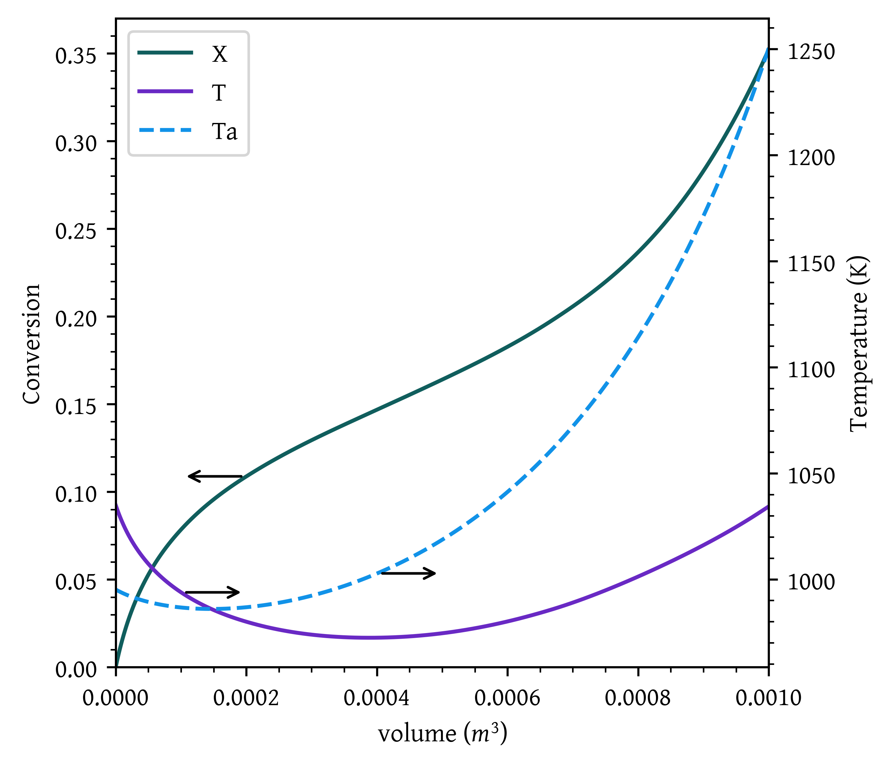

Countercurrent exchange: conversion and temperature

References

Green, Don W., and Marylee Z. Southard, eds. 2019. Perry’s Chemical Engineers’ Handbook. Ninth edition, 85th anniversary edition. New York: McGraw Hill Education.