In class activity: Rate law and stoichiometry

Lecture notes for chemical reaction engineering

Relative rates

1. For the reaction \ce{2A + B -> 3C}, calculate rates of reaction of B and C if -r_A = 10 mol/(dm^3 s)

   Solution

   \frac{r_A}{-a} = \frac{r_B}{-b} = \frac{r_C}{c}

   Rate of disappearance of B = -r_B = \frac{10}{2} = 5 mol/(dm^3 s)

   Rate of production of C = r_C = \frac{10 \times 3}{2} = 15 mol/(dm^3 s)

2. \ce{NO2} is being formed at a rate of 4 mol/(m^3 s) in the reaction \ce{2NO + O2 <=> 2NO2}. Calculate the rate of consumption of \ce{NO}, and \ce{O2}.

   Solution

   \frac{r_{NO}}{-2} = \frac{r_{O_2}}{-1} = \frac{r_{NO_2}}{2}

   Rate of disappearance of \ce{NO} = -r_{NO} = \frac{4 \times 2}{2} = 4 mol/(m^3 s)

   Rate of disappearance of \ce{O2} = -r_{O_2} = \frac{4}{2} = 2 mol/(m^3 s)

Rate law

Determine the rate law for the reaction described in each of the cases below involving species A, B, and C. The rate laws should be elementary as written for reactions that are either of the form \ce{A -> B} or \ce{A + B -> C}.

1. The units of the specific reaction rate are k = \left[\frac{dm^3}{mol \ h} \right].
2. The units of the specific reaction rate are k = \left[\frac{mol}{kg-cat \ h \ (atm)^2} \right].
3. The units of the specific reaction rate are k = \left[\frac{1}{h} \right].
4. The units of a nonelementary reaction rate are k = \left[\frac{mol}{dm^3 \ h} \right].

Solution

1. Second order reaction: -r_A = kC_AC_B

2. Second order gas phase reaction -r'_A = kP_AP_B

3. First order reaction: -r_A = kC_A

4. Second order non elementary reaction -r_A = kC_A^2

Rate law for reversible reaction

For the reaction \ce{C6H6 <=>[{k_B}][{k_{-B}}] C6H4 + H2} (\ce{B <=> D + H2})

determine the rate expression for disappearance of benzene (-r_B). Assume both the forward and reverse reactions are elementary.

Solution

We can write the reactions as two elementary reactions

\ce{B -> D + H2} \cdots (1); \qquad \ce{D + H2 -> B} \cdots (2)

Net rate r_B = -r_{B,1} + r_{B,2}

-r_B = k_B C_B - k_{-B} C_D C_{H_2}

K = \frac{k_B}{k_{-B}}

\therefore -r_B = k_B \left( C_B - \frac{C_D C_{H_2}}{K} \right)

Calculate the activation energy

The decomposition of benzene diazonium chloride to give chlorobenzene and nitrogen

\ce{C6H5N2Cl -> C6H5Cl + N2}

follows first order kinetics. The rate constant data at different temperatures is given in Table 1. Calculate the activation energy.

Table 1: Rate constant data

k (s^{-1})	0.00043	0.00103	0.00180	0.00355	0.00717
T (K)	313.0	319.0	323.0	328.0	333.0

Solution

k = A e^{\frac{-E}{RT}}

Linearize by taking log on both sides

\ln k = \ln A - \left( \frac{E}{R} \right) \left( \frac{1}{T} \right)

The plot of \ln(k) vs. 1/T is linear with a slope of -E/R

import numpy as np
import matplotlib.pyplot as plt
from scipy.stats import linregress

k = np.array([0.00043, 0.00103, 0.00180, 0.00355, 0.00717])
T = np.array([313.0, 319.0, 323.0, 328.0, 333.0])

R = 8.314 # J/mol K

ln_k = np.log(k)
inv_T = 1 / T

slope, intercept, r_value, p_value, std_err = linregress(inv_T, ln_k)
line = slope * inv_T + intercept

activation_energy = -slope*R/1000 # (kJ/mol)

# Plot 
plt.scatter(inv_T, ln_k, color='blue', label='Data points')
plt.plot(inv_T, line, color='red', label='Fit line')

# Labels and title
plt.xlabel('1/T (1/K)')
plt.ylabel('ln(k)')
plt.title('Linear Fit of ln(k) vs 1/T')
plt.legend()

slope_text = f'Slope: {slope:.5e}'
intercept_text = f'Intercept: {intercept:.5e}'
e_text = f'Activation Energy: {activation_energy:.2f} kJ/mol'
plt.annotate(f'{slope_text}\n{intercept_text}\n{e_text}', xy=(0.05, 0.20), xycoords='axes fraction', verticalalignment='top')

# Show plot
plt.show()

Calculate the equilibrium conversion for gas phase reaction, X_e

Consider the following elementary reaction with K_C = 20 dm^3/mol and C_{A0} = 0.2 mol/dm^3. Find X_e for both a batch reactor.

Reaction: \ce{2A <=> B}

Rate law: -r_A = k_A \left[ C_A^2 - \frac{C_B}{K_C} \right]

Solution

Rate law: -r_A = k_A \left[ C_A^2 - \frac{C_B}{K_C} \right]

At equilibrium -r_A \equiv 0 \equiv k_A \left[ C_A^2 - \frac{C_B}{K_C} \right]

K_c = \frac{C_{Be}}{C_{Ae}^2}

stoichiometry:

\ce{A -> 1/2B}

Setting up stoichiometric table

Species	Initial	Change	Remaining
A	N_{A0}	-N_{A0}X	N_A = N_{A0}(1 - X)
B	0	+N_{A0}X/2	N_B = N_{A0} X/2
Total	N_{T0} = N_{A0}		N_T = N_{A0} - N_{A0}X/2

Constant Volume: V = V_0

C_A = \frac{N_A}{V} = C_{A0}(1-X)

C_B = \frac{N_B}{V} = \frac{C_{A0}X}{2}

K_c = \frac{C_{Be}}{C_{Ae}^2} = \frac{C_{A0}\frac{X_e}{2}} {C_{A0}^2(1-X)^2}

2 K_c C_{A0}= \frac{X_e}{(1-X)^2}

2 \times 20 \times 0.2 = \frac{X_e}{(1-X)^2}; \qquad 8 X_e^2 - 17 X_e + 8 = 0

Solving:

Equilibrium conversion: X_e = 0.7

Repeat the calculations above for a flow reactor

Solution

With the flow reactor, we will need to consider changes in molar flow rate as this is a gas phase reaction.

Rate law: -r_A = k_A \left[ C_A^2 - \frac{C_B}{K_C} \right]

At equilibrium -r_A \equiv 0 \equiv k_A \left[ C_A^2 - \frac{C_B}{K_C} \right]

K_c = \frac{C_{Be}}{C_{Ae}^2}

stoichiometry:

\ce{A -> 1/2B}

Stoichiometric table is same as the batch system with moles replaced by molar flow rates.

Species	Entering	Change	Exiting
A	F_{A0}	-F_{A0}X	F_A = F_{A0}(1 - X)
B	0	+F_{A0}X/2	F_B = F_{A0} X/2
Total	F_{T0} = F_{A0}		F_T = F_{A0} - F_{A0}X/2

C_{Ae} = \frac{C_{A0}(1-X_e)}{(1 + \epsilon X_e)}

C_{Be} = \frac{C_{A0}X_e}{2(1 + \epsilon X_e)}

K_{C} = \frac{\frac{C_{A0}X_{e}}{2(1+\epsilon X_{e})}} {\left[\frac{C_{A0}(1-X_{e})}{(1+\epsilon X_{e})}\right]^{2}} = \frac{X_{e}(1+\epsilon X_{e})} {2C_{A0}(1-X_{e})^{2}}

K_c = \frac{C_{Be}}{C_{Ae}^2} = \frac{X_e (1 + \epsilon X_e)}{2 C_{A0}(1-X_e)^2}

2 K_c C_{A0}= \frac{X_e + \epsilon X_e^2)}{(1-2 X_e + X_e^2)} = 8

\epsilon = y_{A0} \delta = 1 \left( \frac{1}{2} - 1 \right) = - \frac{1}{2}

8 = \frac{X_e + 0.5 X_e^2)}{(1-2 X_e + X_e^2)}

Solving for X_e:

Equilibrium conversion: X_e = 0.757

Saponification reaction

The saponification for the formation of soap is:

\ce{3NaOH + (C17H35COO)3C3H5 -> 3C17H35COONa + C3H5(OH)3}

Letting X represent the conversion of NaOH set up a stoichiometric table expressing the concentration of each species in terms of the initial concentration of NaOH and the conversion of X.

Solution

\ce{3NaOH + (C17H35COO)3C3H5 -> 3C17H35COONa + C3H5(OH)3}

\ce{A + 1/3 B -> C + 1/3 D}

C_A = \frac{N_A}{V} = \frac{N_A}{V_0} = N_{A0}(1 - X) = C_{A0}(1 - X)

\Theta_B = \frac{C_{B0}}{C_{A0}}, \quad \Theta_C = \frac{C_{C0}}{C_{A0}}, \quad \Theta_D = \frac{C_{D0}}{C_{A0}}

Species	Symbol	Initially	Change	Remaining	Concentration
NaOH	A	N_{A0}	-N_{A0}X	N_{A0}(1 - X)	C_{A0}(1 - X)
(C_{17}H_{35}COO)_3C_3H_5	B	N_{B0}	-\frac{1}{3}N_{A0}X	N_{A0}\left(\Theta_B - \frac{X}{3}\right)	C_{A0}\left(\Theta_B - \frac{X}{3}\right)
C_{17}H_{35}COONa	C	N_{C0}	N_{A0}X	N_{A0}(\Theta_C + X)	C_{A0}(\Theta_C + X)
C_3H_5(OH)_3	D	N_{D0}	\frac{1}{3}N_{A0}X	N_{A0}\left(\Theta_D + \frac{X}{3}\right)	C_{A0}\left(\Theta_D + \frac{X}{3}\right)
Water (inert)	I	N_{I0}	—	N_{I0}	C_{I0}
Totals		N_{T0}	0	N_T = N_{T0}

Determining C_j = h_j(X) for a Gas-Phase Reaction

A mixture Of 28% \ce{SO2} and 72% air is charged to a flow reactor in which \ce{SO2} is oxidized.

\ce{2SO2 + O2 -> 2 SO3}

1. First, set up a stoichiometric table using only the symbols (i.e., \Theta_i, F_i).

2. Next, prepare a second table evaluating the species concentrations as a function of conversion for the case when the total pressure is 1485 kPa (14.7 atm) and the temperature is constant at 227 °C.

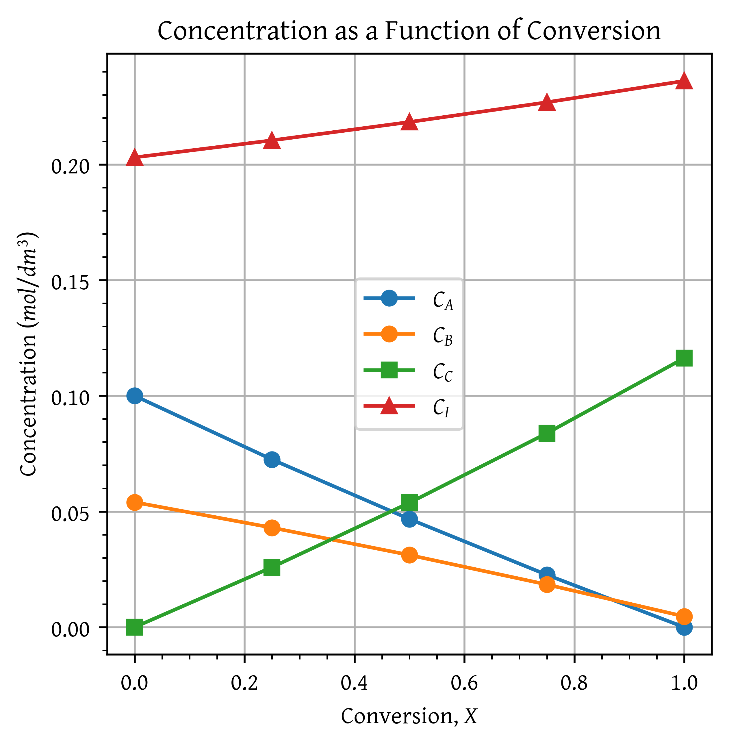
3. Evaluate the parameters and make a plot of each of the concentrations \ce{SO2}, \ce{SO3}, \ce{N2} as a function of conversion

Solution

\ce{2SO2 + O2 -> 2 SO3}

Take \ce{SO2} as basis of calculation

\ce{SO2 + 1/2 O2 -> SO3}

Stoichiometric table

Species	Symbol	Entering	Change	Leaving
SO_2	A	F_{A0}	-F_{A0}X	F_A = F_{A0}(1 - X)
O_2	B	F_{B0} = \Theta_B F_{A0}	-\frac{F_{A0}X}{2}	F_B = F_{A0}\left(\Theta_B - \frac{1}{2}X\right)
SO_3	C	0	+F_{A0}X	F_C = F_{A0}X
N_2	I	F_{I0} = \Theta_I F_{A0}	—	F_I = F_{I0} = \Theta_I F_{A0}
Totals		F_{T0}	-\frac{F_{A0}X}{2}	F_T = F_{T0} - \frac{F_{A0}X}{2}

Concentration:

C_A = \frac{F_A}{\upsilon} = \frac{F_{A0}(1 - X)}{\upsilon}

volumetric flow rate:

\upsilon = \upsilon_0(1 + \epsilon X) \left( \frac{P_0}{P} \right) \left( \frac{T}{T_0} \right)

Neglecting pressure drop in the reaction, and for isothermal reactions:

\upsilon = \upsilon_0(1 + \epsilon X)

C_A = \frac{F_{A0}(1 - X)}{\upsilon_0(1 + \epsilon X)} = C_{A0} \frac{1 - X}{1 + \epsilon X}

Similarly for B

C_B = C_{A0} \frac{\left( \Theta_B - \frac{b}{a}X \right)}{1 + \epsilon X} = \frac{C_{A0}\left(\Theta_B - \frac{1}{2}X\right)}{1 + \epsilon X}

C_T = C_{T0} = \frac{P_0}{RT_0} = \frac{1485}{8.314 \times 500} = 0.357 \frac{mol}{dm^3}

\epsilon = y_{A0} \delta = 0.28 \times ( 1 - 1 - \frac{1}{2}) = -0.14

Initially, 72% of the total number of moles is air containing 21% \ce{O2} and 79% \ce{N2}, along with 28% \ce{SO2}.

F_{A0} = (0.28)(F_{T0})

F_{B0} = (0.72)(0.21)(F_{T0})

\Theta_B = \frac{F_{B0}}{F_{A0}} = \frac{(0.72)(0.21)}{0.28} = 0.54

\Theta_1 = \frac{F_{I0}}{F_{A0}} = \frac{(0.72)(0.79)}{0.28} = 2.03

Substituting for C_{A0} and \epsilon in the species concentrations:

SO_{2}: \quad C_A = C_{A0} \left( \frac{1 - X}{1 + \epsilon X} \right) = 0.1 \left( \frac{1 - X}{1 - 0.14X} \right) \quad \text{mol/dm}^3

O_2: \quad C_B = C_{A0} \left( \frac{\Theta_B - \frac{1}{2}X}{1 + \epsilon X} \right) = 0.1 \left( \frac{0.54 - 0.5X}{1 - 0.14X} \right) \quad \text{mol/dm}^3

SO_3: \quad C_C = \frac{C_{A0}X}{1 + \epsilon X} = \frac{0.1X}{1 - 0.14X} \quad \text{mol/dm}^3

N_2: \quad C_I = \frac{C_{A0}\Theta_1}{1 + \epsilon X} = \frac{(0.1)(2.03)}{1 - 0.14X} \quad \text{mol/dm}^3

import numpy as np
import matplotlib.pyplot as plt

# Constants
C_A0 = 0.1  # mol/dm^3
epsilon = -0.14  # unitless
Theta_B = 0.54  # unitless
Theta_I = 2.03  # unitless

# Conversion range from 0 to 1 with 0.25 interval
X_values = np.arange(0, 1.01, 0.25)

# Concentration calculations
def calculate_concentrations(X, C_A0, epsilon, Theta_B, Theta_I):
    C_A = C_A0 * ((1 - X)/(1 - epsilon * X))
    C_B = C_A0 * ((Theta_B - 0.5 * X) / (1 + epsilon * X))
    C_C = C_A0 * X / (1 + epsilon * X)
    C_I = C_A0 * Theta_I / (1 + epsilon * X)
    return C_A, C_B, C_C, C_I

# Calculate concentrations for each X value
C_A_values, C_B_values, C_C_values, C_I_values = [], [], [], []
for X in X_values:
    C_A, C_B, C_C, C_I = calculate_concentrations(X, C_A0, epsilon, Theta_B, Theta_I)
    C_A_values.append(C_A)
    C_B_values.append(C_B)
    C_C_values.append(C_C)
    C_I_values.append(C_I)

# Plotting the results
plt.plot(X_values, C_A_values, marker='o', label=r'$C_A$')
plt.plot(X_values, C_B_values, marker='o', label=r'$C_B$')
plt.plot(X_values, C_C_values, marker='s', label=r'$C_C$')
plt.plot(X_values, C_I_values, marker='^', label=r'$C_I$')

plt.xlabel('Conversion, $X$')
plt.ylabel('Concentration ($mol/dm^3$)')
plt.title('Concentration as a Function of Conversion')
plt.legend()
plt.grid(True)
plt.show()

Note that Concentration of N_2 (C_I)$ changes with conversion even though nitrogen does not participate in the reaction.

Liquid phase first order reaction

Orthonitroanaline (an important intermediate in dyes—called fast orange) is formed from the reaction of orthonitrochlorobenzene (ONCB) and aqueous ammonia. The liquid-phase reaction is first order in both ONCB and ammonia with k = 0.0017 \ m^3 /kmol \cdot min at 188 \ ^{\circ}C with E = 11273 \ cal/mol. The initial entering concentrations of ONCB and ammonia are 1.8 \ kmol/m^3 and 6.6 \ kmol/m^3, respectively.

\ce{C6H4ClNO2 + 2 NH3 -> C6H6N2O2 + NH4Cl}

1. Set up a stoichiometric table for this reaction for a flow system.

2. Write the rate law for the rate of disappearance of ONCB in terms of concentration.

3. Explain how parts (a) and (b) would be different for a batch system.

4. Write -r_A solely as a function of conversion. -r_A = ______

5. What is the initial rate of reaction (X = 0)

   at 188 \ ^{\circ}C? -r_A = ______

   at 25 \ ^{\circ}C? -r_A = ______

   at 288 \ ^{\circ}C? -r_A = ______

6. What is the rate of reaction when X = 0.90

   at 188 \ ^{\circ}C? -r_A = ______

   at 25 \ ^{\circ}C? -r_A = ______

   at 288 \ ^{\circ}C? -r_A = ______

7. What would be the corresponding CSTR reactor volume at 25 \ ^{\circ}C to achieve 90% conversion and at 288 \ ^{\circ}C for a feed rate of 2 \ dm^3 /min

   at 25 \ ^{\circ}C? V = ______

   at 288 \ ^{\circ}C? V = ______

Solution

\ce{C6H4ClNO2 + 2 NH3 -> C6H6N2O2 + NH4Cl}

\ce{A + 2 B -> C + D}; -r_A = k C_A C_B

Problem data

k	0.0017 m^3/kmol min at \ 188 ^\circ C
E	11273 cal/mol
$C_A	1.8 kmol/m^3
$C_B	6.6 kmol/m^3

1. Stoichiometric table for flow reactor

Species	Entering	Change	Exiting
A	F_{A0}	-F_{A0}X	F_A = F_{A0}(1 - X)
B	F_{B0} = \Theta_B F_{A0}	-2 F_{A0}X	F_B = F_{A0}(\Theta_B - 2X)
C	0	F_{A0}X	F_C = F_{A0} X
D	0	F_{A0}X	F_D = F_{A0} X

\Theta_B = \frac{6.6}{1.8} = 3.67

2. -r_A = k C_A C_B

3. For batch system

C_A = \frac{N_A}{V}

The stoichiometric table needs to be set up in terms of N instead of F. The reaction rate expression would remain same.

4. -r_A as a function of conversion

-r_A = k C_A C_B

C_A = C_{A0}(1-X)

C_B = C_{A0}(\Theta_B - 2X)

-r_A = k C_{A0}(1-X) C_{A0}(\Theta_B - 2X)

-r_A = k C_{A0}^2 (1-X)(\Theta_B - 2X)

5. Initial rates of reaction

k at different temperatures

k = k_0 exp \left[ \frac{E}{R} \left( \frac{1}{T_0} - \frac{1}{T} \right)\right]

T (°C)	k (m^3/kmol min)
25 (298K)	2.03 \times 10^{-6}
188 (461K)	0.0017
288 (561K)	0.152

1. At 188 °C

-r_A = k C_{A0}^2 \Theta_B = 0.0017 \times (1.8)^2 \times 3.67 = 0.0202 \ kmol/m^3 min

2. At 25 °C: 2.41 \times 10^{-5} \ kmol/m^3 min

3. At 288 °C: 0.1806 kmol/m^3 min

6. rates of reaction at X = 0.9

-r_A = k C_{A0}^2 (1 - X)(\Theta_B - 2X)

1. At 188 °C: 0.00103 kmol/m^3 min

2. At 25 °C: 1.23 \times 10^{-6} kmol/m^3 min

3. At 288 °C: 0.0092 kmol/m^3 min

7. CSTR Volume

X = 90% = 0.9; \upsilon_0 = 2 dm^3/min

F_{A0} = C_{A0} \upsilon_0 = 3.6 mol/min

1. V at 25 °C

   V = \frac{F_{A0}X}{-r_A|_{exit}}

   V = 2634.1 m^3

2. V at 288 °C: 352 m^3