Distribution of residence time

Chemical Reaction Engineering

General Considerations

• Models developed so far are for perfectly mixed batch reactor, the plug flow tubular reactor, packed bed reactor, and perfectly mixed continuous tank reactor.

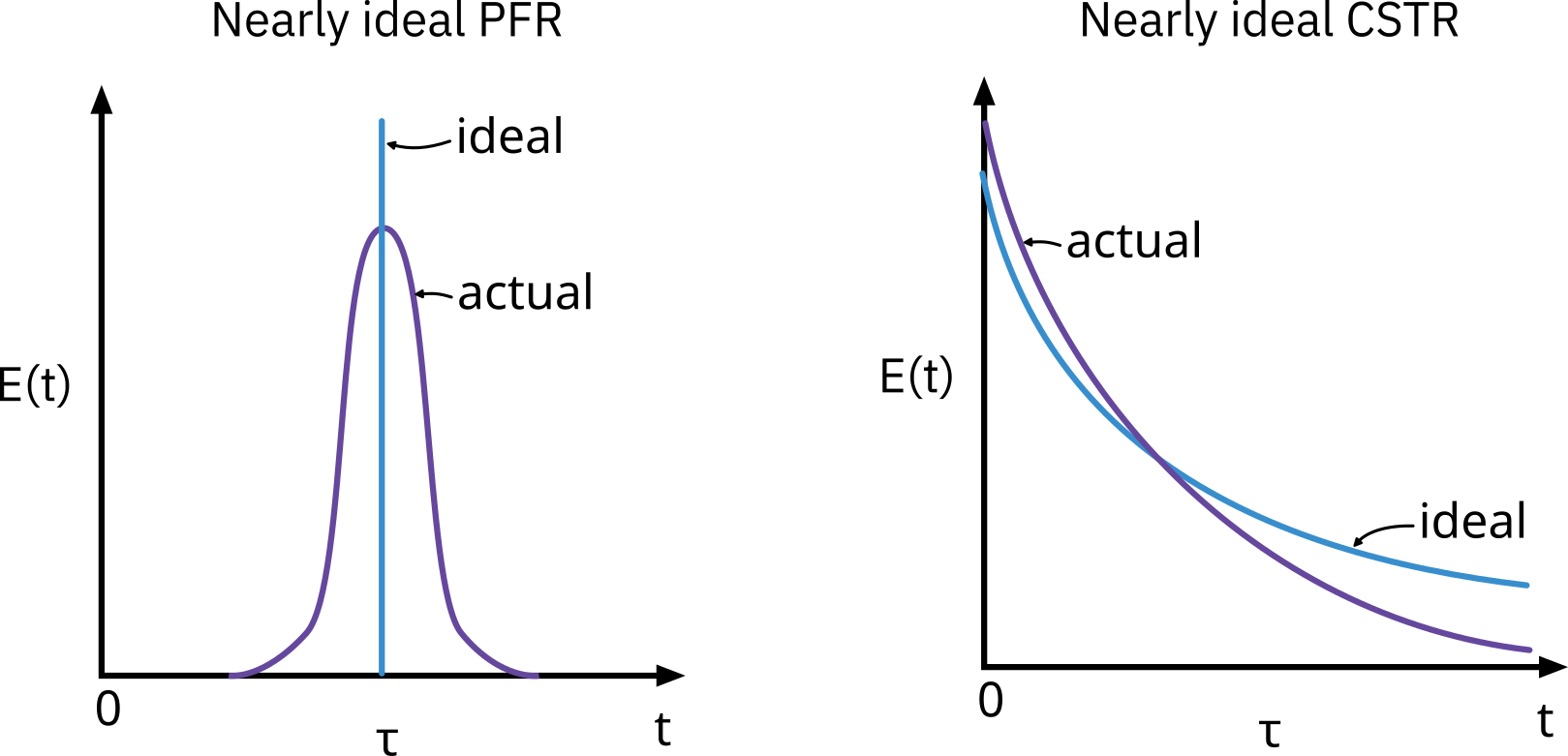
• Real world behavior is often very different from the ideal behavior.

• Use residence time distribution to analyze and characterize non-ideal reactors.

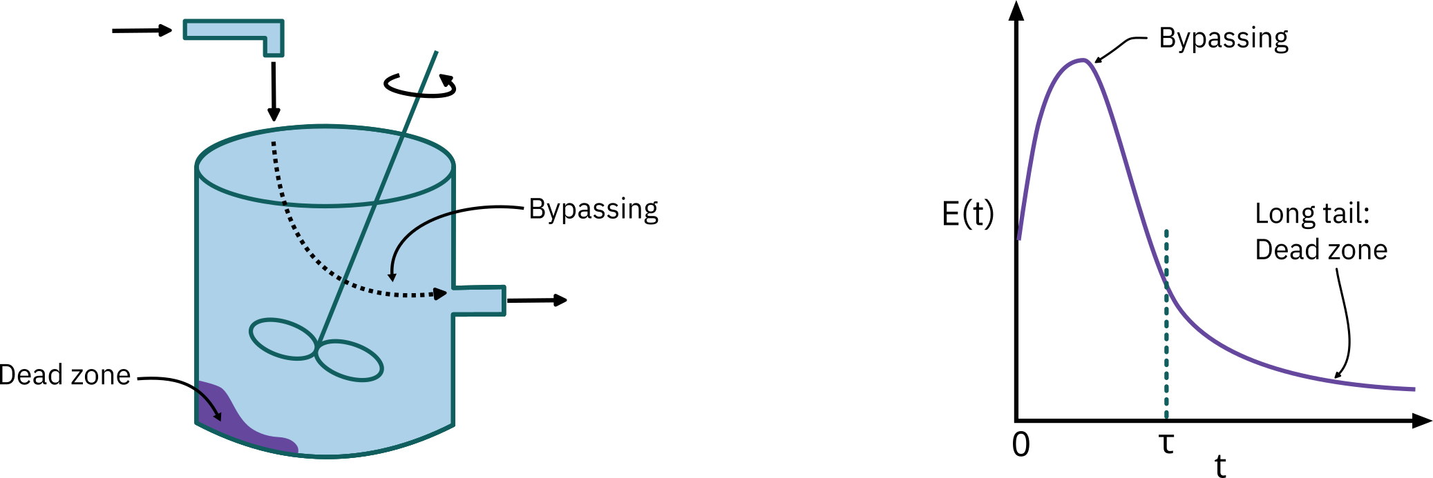
  • diagnose problems of reactor operations

  • predict conversion in existing reactor when new chemical reaction is used in the reactor.

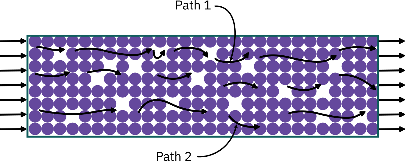
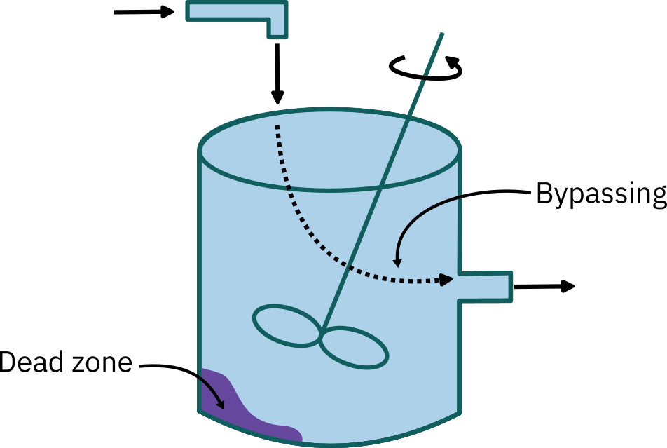
Examples of non-ideality

• Describing deviation from ideal reactor mixing pattern

  • Residence time distribution (RTD)
  • Quality of mixing
  • Model used to describe the system

• Residence time distribution (RTD) function

  Popularized by Prof. P. V. Dankwerts

Residence Time Distribution (RTD) function

Residence time: The time atoms have spent in the reactor.

• Plug flow reactor: Atoms spend exactly the same time in these two reactors.

• Ideal batch reactor: Atoms spend exactly the same time in these two reactors.

• CSTR: Feed introduced into a CSTR becomes completely mixed with the material already in the reactor.

  • Some atoms entering the CSTR leave almost immediately.
  • Other atoms remain in the reactor almost forever as all the material recirculates within the reactor and is virtually never removed from the reactor at one time.

• Distribution of residence times can significantly affect reactor performance.

  • The RTD is a characteristic of the mixing that occurs in the chemical reactor.

  • RTD yields distinctive clues to the type of mixing occurring within it and is one of the most informative characteristics of the reactor.

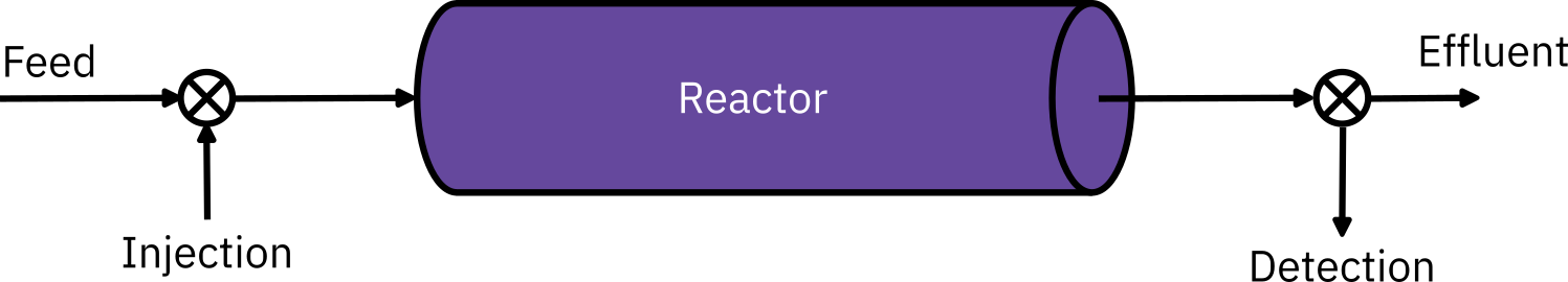
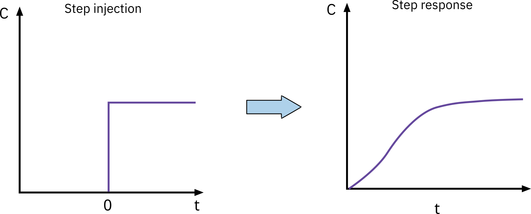
Measurement of the RTD

• Determined experimentally
  • Injecting tracer into the reactor at some time t=0 and then measuring the tracer concentration C in the effluent stream as a function of time.

• Properties of Tracer
  • Inert (non-reactive)
  • Easily detectable
  • Similar physical properties to the reacting mixture
  • Completely soluble in the reacting mixture
  • Does not adsorb on reactor walls
  • Tracer behavior should mimic the behavior of material flowing in the reactor.
• Common tracers: colored dye, radioactive material, inert gases

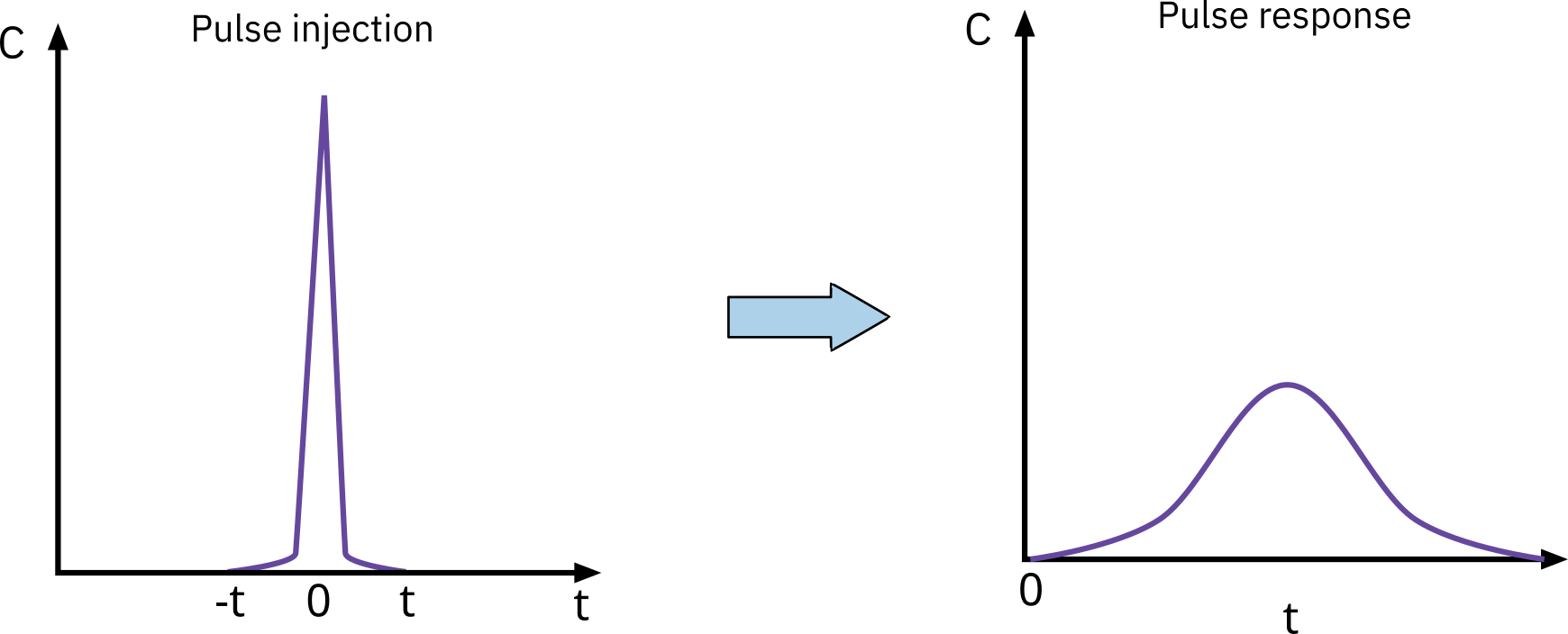
Pulse input experiment

• An amount of tracer N_0 is suddenly injected in one shot into the feed stream.

• Outlet concentration is measured with time.

• Consider single-input and single-output system:

  • Only flow carries the tracer material.
  • No dispersion.
  • Increment of time \Delta t is sufficiently small that the concentration of tracer C(t) exiting between t and t + \Delta t is essentially the same.

• Amount of tracer material leaving the reactor between t and (t + \Delta t): \Delta N = C(t) \cdot \upsilon \cdot \Delta t \quad \text{where } \upsilon \text{ is the volumetric flow rate} \tag{1}

Pulse input experiment

• Dividing by the Total Amount of Material that was Injected

\frac{\Delta N}{N_0} = \frac{\upsilon C(t)}{N_0} \Delta t \tag{2}

\Rightarrow Fraction of material that has residence time in the reactor between t and t + \Delta t

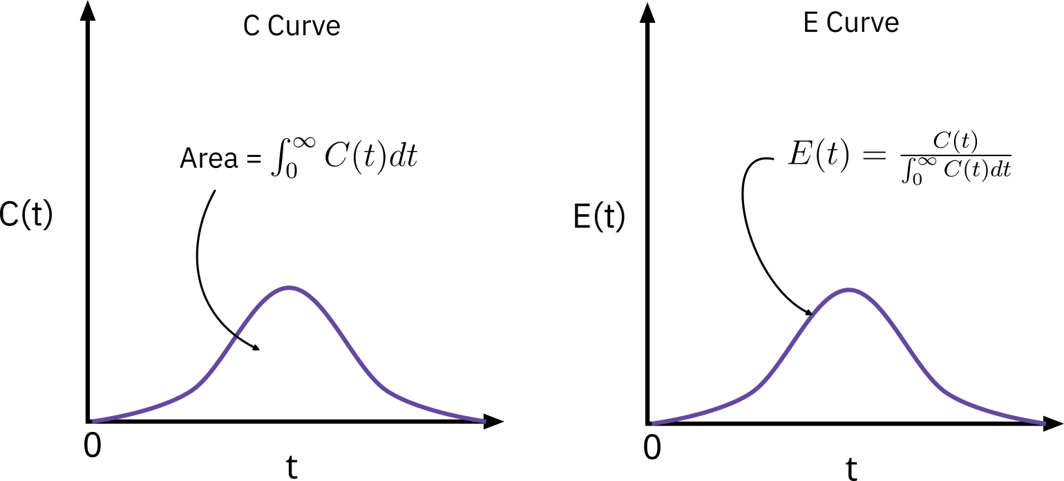
• For pulse injection let

E(t) = \frac{\upsilon C(t)}{N_0} \quad \text{... Residence time function}

• Residence time function

  Function that describes in a quantitative manner how much time different fluid elements have spent in the reactor

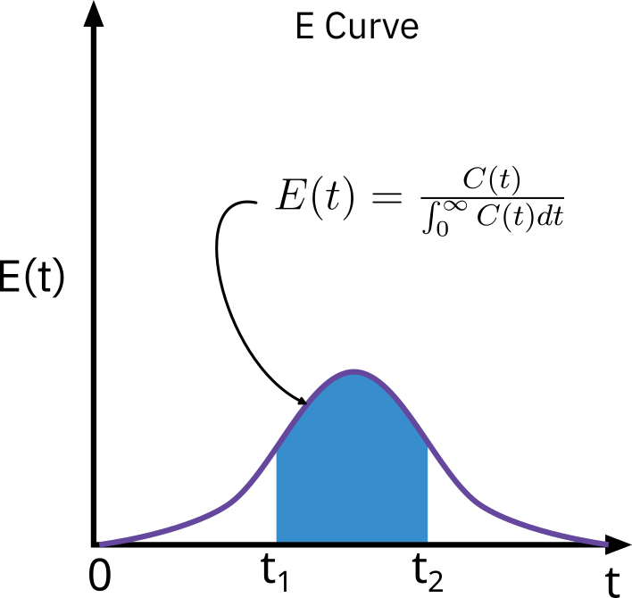
\therefore \frac{\Delta N}{N_0} = E(t) \Delta t

Pulse input experiment

• E(t) dt is the fraction of fluid exiting the reactor that has spent between time t and t + \Delta t inside the reactor.

• If N_0 is not known directly, it can be obtained from the outlet concentration measurements by summing up all the amounts from 0 \text{ to } \infty

• Writing Equation 1 in Differential Form

  dN = \upsilon C(t) dt

• Integrating

  N_0 = \int_{0}^{\infty} \upsilon C(t) dt

  \upsilon is usually constant, therefore

  E(t) = \frac{C(t)}{\int_{0}^{\infty} C(t) dt} \tag{3}

  • E(t) is also called exit age distribution function

Pulse input experiment

• The E curve is just the C curve divided by the area under the C curve.

Pulse input experiment

• Fraction of material leaving the reactor that has resided in the reactor between t_1 and t_2

  = \int_{t_1}^{t_2} E(t) \, dt

• Fraction of all material that has resided for a time t in the reactor between t = 0 and t = \infty is 1

  \int_{0}^{\infty} E(t) \, dt = 1

Difficulties with pulse technique

• Obtaining a reasonable pulse at the reactor entrance
  • Injection time should be very short compared to residence times in various segments of the reactor.
  • There must be negligible dispersion between the point of injection and the entrance to the reactor.
• If these conditions are achieved, pulse technique is a simple and direct way to obtain RTD.

Step tracer experiment

• Inlet is either:

  • Perfect pulse input (Dirac delta function)
  • Imperfect pulse, determine E(t)

• Cumulative distribution F(t) can be determined from step input.

• Cumulative distribution gives the fraction of material F(t) that has been in the reactor at time t or less.

Step tracer experiment

• Consider constant tracer addition to a feed that is initiated at t = 0

C_{\text{in}}(t) = \begin{cases} 0 & t < 0 \\ C_0, \text{constant} & t \ge 0 \end{cases}

• The concentration of tracer in feed is kept at this level until the concentration in the effluent is almost the same as the feed.

• As inlet concentration is constant with time, C_0, we can take it out of the integral sign:

C_{\text{out}}(t) = C_0 \int_{0}^{t} E(t') dt'

• Dividing by t_0:

\left[ \frac{C_{\text{out}}(t)}{C_0} \right]_{\text{step}} = \int_{0}^{t} E(t') dt' = F(t)

Step tracer experiment

F(t) = \left[ \frac{C_{\text{out}}(t)}{C_0} \right]_{\text{step}} \tag{4}

• We differentiate Equation 4 to obtain RTD function:

E(t) = \frac{dF}{dt} = \frac{d}{dt} \left[ \frac{C_{\text{out}}(t)}{C_0} \right]_{\text{step}}

• Positive step is usually easier to carry out experimentally than the pulse test.

• Total amount of tracer in feed over the period of test does not have to be known

• Drawbacks

  • It may be difficult to maintain constant tracer concentration in the feed.
  • Obtaining RTD involves differentiation of the data. ( differentiation can lead to large errors. )
  • A large amount of tracer is required.

• Other Tracer Techniques

  • Negative step (elution), Frequency response method, Methods that use inputs other than pulse or step

  • These techniques are much more difficult to carry out and are not encountered often.

Integral relationships

Sometimes F curve is used in the same manner as the RTD in modeling chemical reactors.

• Fraction of effluent that has been in the reactor for less than t

  F(t) = \int_{0}^{t} E(t) \, dt

• Fraction of effluent that has been in the reactor for longer than t

  1 - F(t) = \int_{t}^{\infty} E(t) \, dt

Mean residence time

• First moment of the RTD function

t_m = \frac{\int_0^\infty t E(t) dt}{\int_0^\infty E(t) dt} = \int_0^\infty t E(t) dt

• In absence of dispersion, and for constant volumetric flow rate,

  t_m = \tau \qquad \Rightarrow \qquad V = \upsilon t_m \qquad \text{ only for closed systems }

Other moments of RTD

• Variance (\sigma^2): Magnitude indicates spread of distribution

  \sigma^2 = \int_0^\infty (t - t_m)^2 E(t) dt

• Skewness (s^3): Magnitude measures extent that distribution is skewed in one direction in reference to mean

  s^3 = \frac{1}{\sigma^{3/2}} \int_0^\infty (t - t_m)^3 E(t) dt

Normalized RTD function

• Frequently a normalized function is used instead of E(t).

• Let \theta \equiv \frac{t}{\tau} : Number of reactor volumes of fluid based on entrance conditions that have flowed through the reactor in time t

  E(\theta) = \tau E(t) \qquad; \qquad \int_{0}^{\infty} E(\theta) d\theta = 1

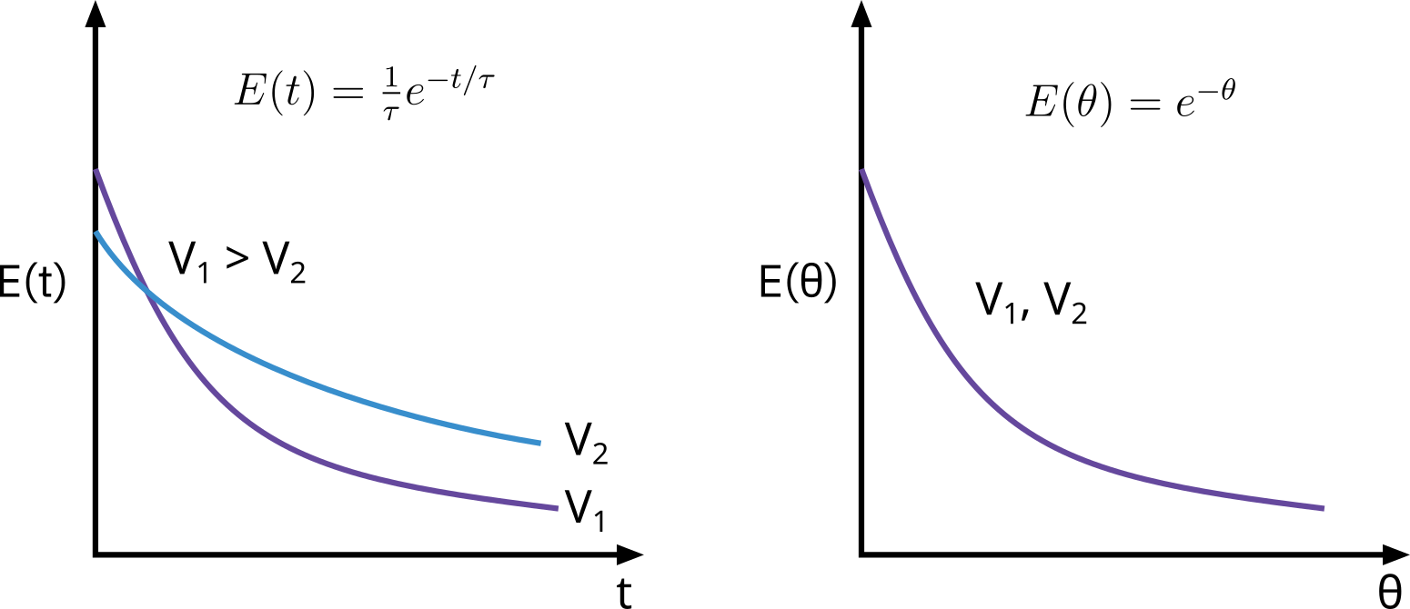
• The flow performance inside reactors of different sizes can be compared directly.

• If normalized function E(\Theta) is used, all perfectly mixed CSTRs have numerically the same RTD. If the simple function E(t) is used, numerical values of E(t) can differ substantially.

Internal-age distribution I(\alpha)

• A function such that I(\alpha) \Delta \alpha is the fraction of material inside the reactor that has been inside for a period of time between \alpha and \alpha + \Delta \alpha.

• In catalytic reaction using catalyst whose activity decays with time, I(\alpha) is of importance and can be used to model the reactor.

  I(\alpha) = \frac{(1 - F(\alpha))}{\tau}

  E(\alpha) = -\frac{d}{d\alpha} \left[ \tau I(\alpha) \right]

• For CSTR

  I(\alpha) = -\frac{1}{\tau} e^{-\alpha / \tau}

RTD in ideal reactors: batch and PFR

• E(t) = \delta(t - \tau) (Dirac delta function)

  \delta(x) = \begin{cases} 0 & \text{when } x \neq 0 \\ \infty & \text{when } x = 0 \end{cases}

• Properties of Dirac delta function

\int_{-\infty}^{\infty} \delta(x) dx = 1 \qquad ; \qquad \int_{-\infty}^{\infty} g(x) \delta(x - \tau) dx = g(\tau)

• Mean Residence Time

t_m = \int_{0}^{\infty} t E(t) dt = \int_{0}^{\infty} t \delta(t - \tau) dt = \tau

• Variance \sigma^2 = \int_{0}^{\infty} (t - \tau)^2 \delta(t - \tau) dt = 0

• Variance Calculation

  • The variance \sigma^2 measures the spread of residence times around the mean residence time \tau.

  • For an ideal plug flow reactor, there is no spread because every particle has the same residence time.

  • Therefore, when calculating the variance using the delta function, the integrand (t - \tau)^2 is zero at t = \tau, and since \delta(t - \tau) is zero everywhere else, the integral evaluates to zero:

    \sigma^2 = \int_{0}^{\infty} (t - \tau)^2 \delta(t - \tau) \, dt = 0

Single-CSTR RTD

• Concentration in effluent stream is identical to the concentration throughout the reactor.

• Material balance on an inert tracer injected as a pulse at t = 0

\text{In} - \text{Out} = \text{Accumulation} \Rightarrow 0 - \upsilon C = V \frac{dC}{dt}

• Initial Condition: \text{at } t = 0 \quad C = C_0

C(t) = C_0 e^{-t/\tau}

• RTD Function

E(t) = \frac{C(t)}{\int_{0}^{\infty} C(t) dt} = \frac{C_0 e^{-t/\tau}}{\int_{0}^{\infty} C_0 e^{-t/\tau} dt} = \frac{e^{-t/\tau}}{\tau}

Single-CSTR RTD

• Normalized RTD Function

E(\theta) = e^{-\theta} \quad \text{where} \quad \theta = \frac{t}{\tau} ; \quad E(\theta) = \tau E(t)

• Cumulative Distribution Function F(t)

  F(t) = \int_{0}^{t} E(t)dt = \int_{0}^{t} \frac{e^{-t/\tau}}{\tau} dt

  F(t) = 1 - e^{-t/\tau}; F(\theta) = 1 - e^{-\theta}

• Mean residence time t_m = \int_{0}^{\infty} t E(t) dt = \int_{0}^{\infty} \frac{t}{\tau} e^{-t/\tau} dt = \tau

  \sigma^2 = \int_{0}^{\infty} \frac{(t - \tau)^2}{\tau} e^{-t/\tau} dt = \tau^2 \int_{0}^{\infty} (x - 1)^2 e^{-x} dx = \tau^2

• \sigma = \tau: Standard deviation is as large as the mean

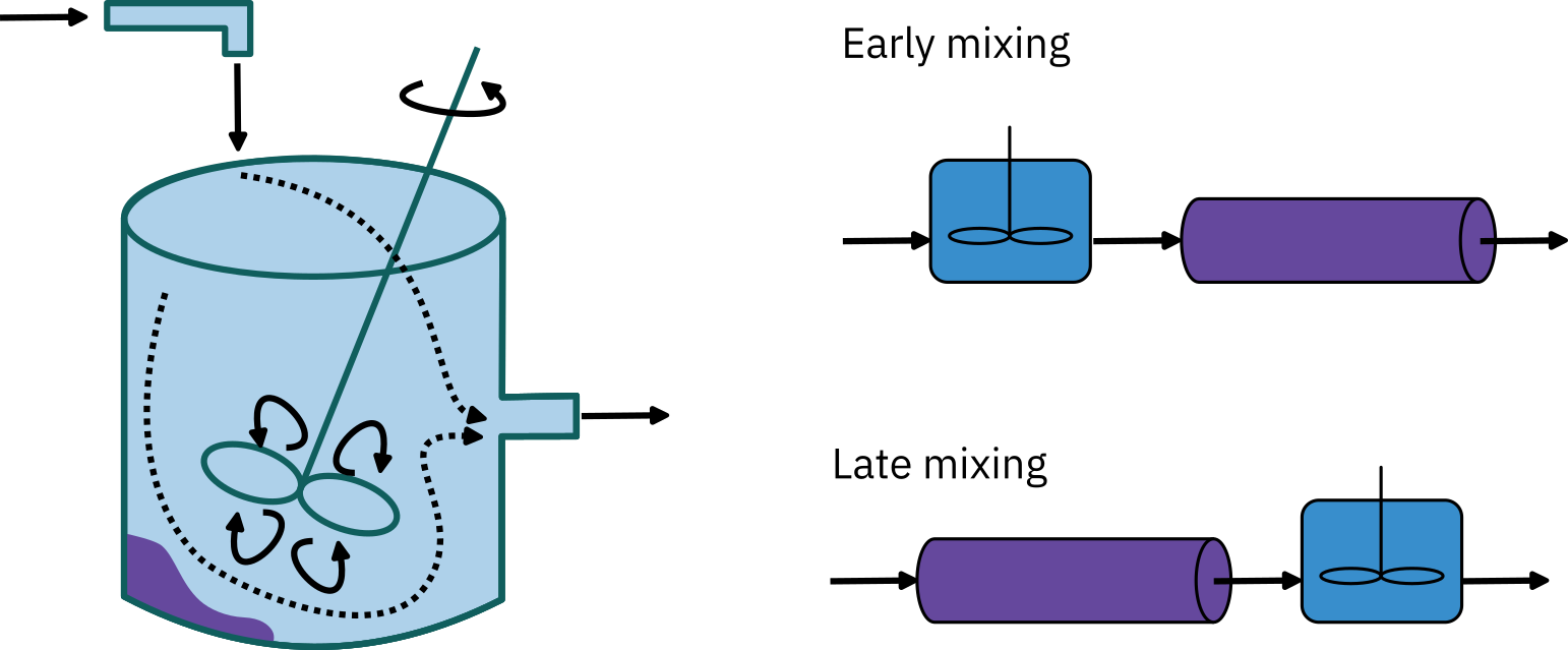
PFR/CSTR series RTD

• In some stirred tanks, there is a highly agitated zone in the vicinity of the impeller \rightarrow CSTR

• Depending on the location of the inlet and outlet, the reacting mixture may follow a tortuous path either before entering or after leaving the perfectly mixed zone \rightarrow PFR

PFR/CSTR series RTD

• Early mixing: C = C_0 e^{-t/\tau_s}; \tau_s: CSTR mean RT; \tau_p: PFR mean RT

  This conc. output will be delayed by \tau_p at the outlet plug flow section

• RTD E(t) = \begin{cases} 0 & t < \tau_p \\ \frac{e^{-(t - \tau_p) / \tau_s}}{\tau_s} & t \ge \tau_p \end{cases}

• Late Mixing

E(t) = \begin{cases} 0 & t < \tau_p \\ \frac{e^{-(t - \tau_p) / \tau_s}}{\tau_s} & t \ge \tau_p \end{cases}

• Exactly same as early mixing
• Even though RTD will be the same for both these cases, conversion can be very different
• RTD is not a complete description of the structure for a particular reactor / reactor systems

Diagnostics and troubleshooting

Diagnostics and troubleshooting