CRE | Chemical Reaction Engineering – Non-isothermal reactor design

Need for energy balance

Consider a liquid phase PFR for a first-order exothermic reaction.

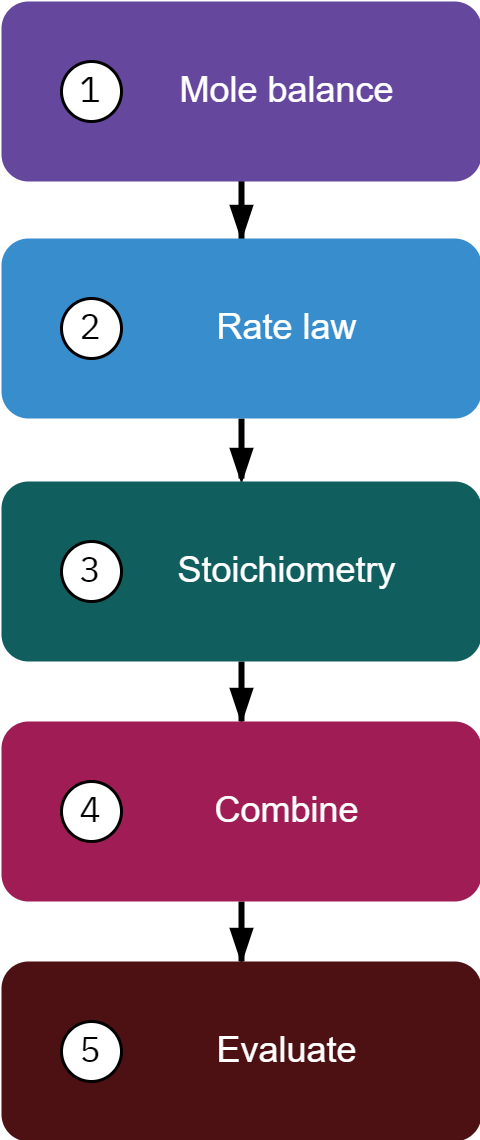
Mole balance

$\frac{dX_A}{dV} = \frac{-r_A}{F_{A0}}$
Rate law

$-r_A = kC_A = -k_0 \exp \left[ \frac{E}{R} \left( \frac{1}{T_1} - \frac{1}{T} \right)\right] C_A$
Stoichiometry

$C_A = C_{A0}(1-X_A)$
Combine: Put $F_{A0}$ in terms of $C_{A0}$

$\frac{dX}{dV} = -k_0 \exp \left[ \frac{E}{R} \left( \frac{1}{T_1} - \frac{1}{T} \right)\right] \frac{(1 - X_A)}{\upsilon_0}$
Evaluate

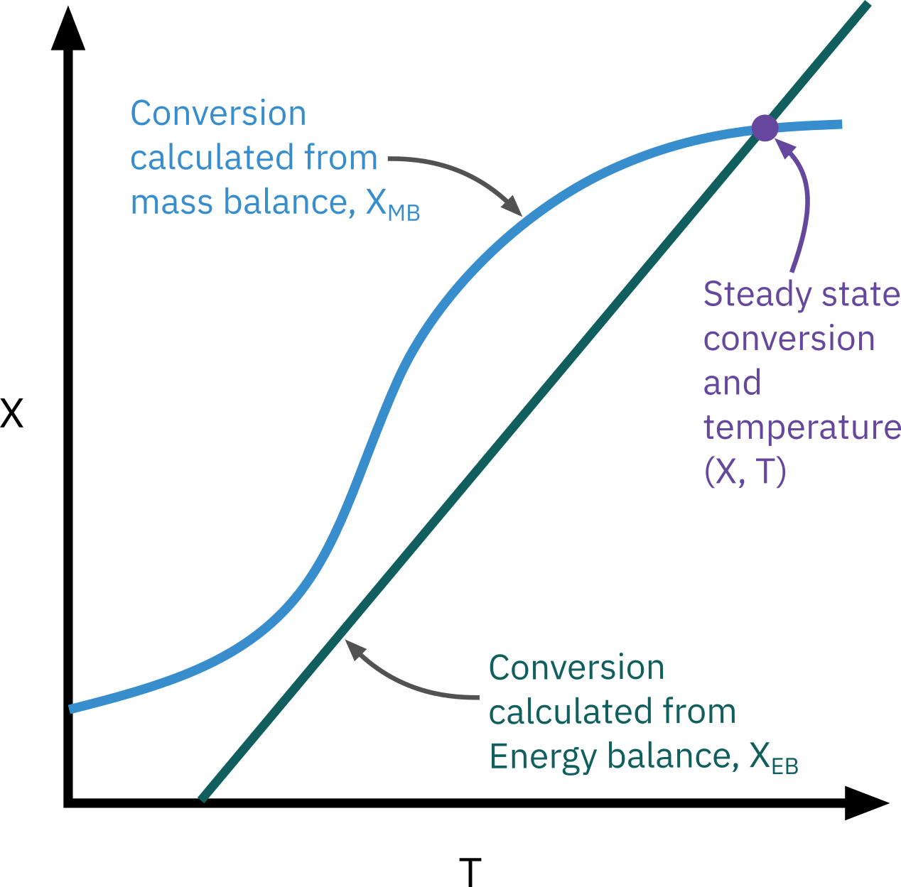
We cannot solve this equation because both $X$ , and $T$ vary with $V$ and we don’t have $X$ either as a function of $V$ or $T$ . We need one more equation

$\Rightarrow$ The energy balance

Thermodynamics in a closed system

First law of thermodynamics

System

A system is any bounded portion of the universe, moving or stationary, which is chosen for the application of the various thermodynamic equations.
Closed system: no mass crosses boundaries

$\begin{aligned} \text{Change in} & & \text{Heat flow} & & \text{Work done by} \\ \text{total energy} &\;\; = & \text{to} \qquad &\;\; - & \text{by the system} \\ \text{of the system} & & \text{the system} & & \text{on the surroundings} \end{aligned}$

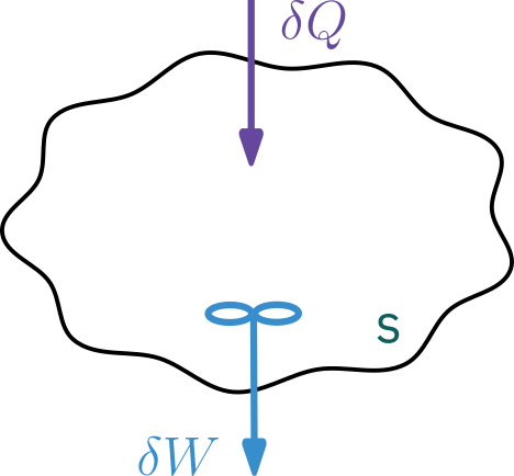
$d \hat{E} = \delta Q - \delta W$

$\hat{E}$ : Change in total energy of the system
$\delta Q$ : Heat flow to the system
$\delta$ : Work done by system on the surroundings

Thermodynamics in an open system

Open system: continuous flow system, mass crosses the system’s boundaries
Mass flow can add or remove energy
System volume is well mixed
$N$ species each entering and leaving at molar flow rate of $F_i$ and has internal energy of $E_i$

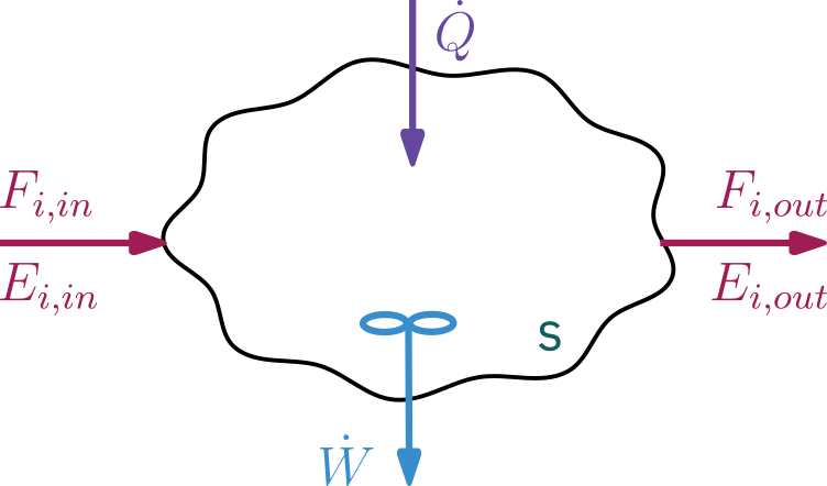
$\begin{aligned} \text{Rate of accumulation} & & & & \text{Work done} & & \text{Energy added} & & \text{Energy leaving} \\ \text{of energy} &\;\; = & \text{Heat in} &\;\; - & \text{by} \qquad &\;\; + & \text{to the system} &\;\; - & \text{the system by} \\ \text{in the system} & & & & \text{the system} & & \text{by mass flow in} & & \text{mass flow out} \end{aligned}$

$\frac{d \hat{E}_{sys}}{dt} = \dot Q - \dot W + \left. \sum_{i=1}^{N} E_i F_i \right|_{in} - \left. \sum_{i=1}^{N} E_i F_i \right|_{out}$

The work term, $\dot W$

$\dot W$ : Rate of work done by the system on the surroundings
- Flow work: work required to get the mass into and out of system
- Other work (shaft work, $\dot W_s$ ): work produced by stirrer or turbine

$\dot{W} =\overbrace{ -\left.\sum_{i=1}^n F_i P \tilde V_i \right|_{in} +\left.\sum_{i=1}^n F_i P \tilde V_i \right|_{out}}^{\color{RoyalBlue}{\text{flow work}}} +\underbrace{\dot W_s}_{\color{RoyalBlue}{\text{shaft work}}}$

$P$ : Pressure; $\tilde V_i$ : Specific molar volume of species $i$
In most instances, the flow-work term is combined with those terms in the energy balance that represent the energy exchange by mass flow across the system boundaries.

$\frac{d \hat{E}_{sys}}{dt} = \dot Q - \dot W_s + \left. \sum_{i=1}^{N} F_i (E_i + P \tilde V_i) \right|_{in} - \left. \sum_{i=1}^{N} F_i (E_i + P \tilde V_i) \right|_{out}$

The energy term, $E_i$

The energy $E_i$ is the sum of the internal energy, the kinetic energy, the potential energy, and any other energies, such as electric or magnetic energy or light

$E_i = U_i + \frac {u_i^2} {2} + g z_i + \text{other}$

Generally in chemical reactors, $U_i \gg {u_i^2}/{2} + g z_i + \text{other}$

$E_i \approx U_i$ : Internal energy is major contributor to energy term.

$\frac{d \hat{E}_{sys}}{dt} = \dot Q - \dot W_s + \left. \sum_{i=1}^{N} F_i (U_i + P \tilde V_i) \right|_{in} - \left. \sum_{i=1}^{N} F_i (U_i + P \tilde V_i) \right|_{out}$

Enthalpy $H_i$ is defined as $H_i = U_i + P \tilde V_i$

$\frac{d \hat{E}_{sys}}{dt} = \dot Q - \dot W_s + \sum_{i=1}^{N} F_{i0} H_{i0} - \sum_{i=1}^{N} F_{i} H_{i}$

Steady state energy balance: conversion

Consider reaction

$\ce{aA + bB -> cC + dD}$

$\ce{A + \frac{b}{a} B -> \frac{c}{a} C + \frac{d}{a} D}$
$F_i = F_{A0}(\Theta_i + \nu_i X)$

$\Theta_i = \frac{F_{i0}}{F_{A0}}$

$\nu_i$ : Stoichiometric coefficient

$F_A = F_{A0}(1 - X)$

$F_B = F_{A0}(\Theta_B - \frac{b}{a} X)$

$F_C = F_{A0}(\Theta_C + \frac{c}{a} X)$

$F_D = F_{A0}(\Theta_D + \frac{d}{a} X)$

$F_I = F_{A0}(\Theta_I)$

Steady state reaction

$\dot Q - \dot W_s + \sum_{i=1}^{N} F_{i0} H_{i0} - \sum_{i=1}^{N} F_{i} H_{i} = 0$

Lets evaluate

$\sum_{i=1}^{N} F_{i0} H_{i0} - \sum_{i=1}^{N} F_{i} H_{i}$

Steady state energy balance: conversion

$\begin{aligned} \sum_{i=1}^{N} F_{i0} H_{i0} - \sum_{i=1}^{N} F_{i} H_{i} = & \;\; F_{A0}\left[ (H_{A0} - H_A) + (H_{B0} - H_B) \Theta_B \right. \\ & \left. + (H_{C0} - H_C) \Theta_C + (H_{D0} - H_D) \Theta_D + (H_{I0} - H_I) \Theta_I \right] \\ &\;\; - \underbrace{ \color{RoyalBlue}{ \left[ \frac{d}{a} H_D + \frac{c}{a} H_C - \frac{b}{a} H_B - H_A \right] }}_{\Delta H_{Rx} \text{at temperature T}} F_{A0} X \\ = &\;\; F_{A0} \sum_{i=1}^{N} (H_{i0} - H_i) - \Delta H_{Rx} F_{A0} X \end{aligned}$

$\dot Q - \dot W_s + F_{A0} \sum_{i=1}^{N} \Theta_i (H_{i0} - H_i) - \Delta H_{Rx} F_{A0} X = 0$

Use this equation when enthalpies are available.
If there is a phase change, we must use this equation for energy balance.
In most cases, the work done $\dot W_s$ is zero

Specific enthalpy $H_i$

Specific enthalpy of species $i$ at a particular temperature and pressure is given by

$H_i = H_i^\circ(T_R) + \Delta H_{Qi}$
- Ignoring enthalpy of mixing
- $H_i^\circ(T_R)$ : Enthalpy of formation of species $i$ at reference temperature $T_R$
- $\Delta H_{Qi}$ : the change in enthalpy that results when the temperature is raised from $T_R$ , to some temperature $T$
In absence of phase change, $\Delta H_{Qi} = \int_{T_1}^{T_2} C_{P_i} dT$
The heat capacity at temperature $T$ is frequently expressed as a quadratic function of temperature

$C_{P_i} = \alpha_i + \beta_i T + \gamma_i T^2$

$H_i = H_i^\circ(T_R) + \int_{T_1}^{T_2} C_{P_i} dT$

Steady state energy balance

Constant heat capacity

Consider constant heat capacity: $\qquad$ $\int_{T_{i0}}^{T} C_{P_i} dT = C_{P_i} \left[ T - T_{i0}\right]$
$H_{i0} = H_i^\circ(T_R) + C_{P_i} \left[ T_{i0} - T_{R} \right]$
$H_{i} = H_i^\circ(T_R) + C_{P_i} \left[ T_{i} - T_{R} \right]$

$H_{i0} - H_i = \left( \cancel{H_i^\circ(T_R)} + C_{P_i} \left[ T_{i0} - \cancel{T_{R}}\right] \right) - \left( \cancel{H_i^\circ(T_R)} + C_{P_i} \left[ T_{i} - \cancel{T_{R}}\right] \right)$

$H_{i0} - H_i = C_{P_i} \left[ T_{i0} - T_{i}\right] = - C_{P_i} \left[ T_{i} - T_{i0}\right]$

$\dot Q - \dot W_s - F_{A0} \sum_{i=1}^{N} \Theta_i C_{P_i} \left[ T_{i} - T_{i0}\right] - \Delta H_{Rx} F_{A0} X = 0$

Heat of reaction, $\Delta H_{Rx}(T)$

For reaction: $\ce{aA + bB -> cC + dD}$
Heat of reaction:

$\Delta H_{Rx}(T) = \frac{d}{a} H_D (T) + \frac{c}{a} H_C (T) - \frac{b}{a} H_B (T) - H_A (T)$

Specific enthalpy of each species

$H_i = C_{P_i} \left[ T - T_{R}\right]$

Substituting

$\begin{aligned} \Delta H_{Rx}(T) = & & \left[ \underbrace{ \frac{d}{a} H_D^\circ (T_R) + \frac{c}{a} H_C^\circ (T_R) - \frac{b}{a} H_B^\circ (T_R) - H_A^\circ (T_R) }_{\color{RoyalBlue}{\Delta H_{Rx}^\circ \text{ at } T_R}} \right] & + & \left[ \underbrace{ \frac{d}{a} C_{P_D} + \frac{c}{a} C_{P_C} - \frac{b}{a} C_{P_B} - C_{P_A} }_{\color{RoyalBlue}{\Delta C_{P}}} \right] \left(T - T_R \right) \end{aligned}$

$\Delta H_{Rx}(T) = \Delta H_{Rx}^\circ(T_R) + \Delta C_{P}(T - T_R)$

Steady state energy balance

Constant heat capacity, adiabatic system

$\dot Q - \dot W_s - F_{A0} \sum_{i=1}^{N} \Theta_i C_{P_i} \left[ T_{i} - T_{i0}\right] - \left[ \Delta H_{Rx}^\circ(T_R) + \Delta C_{P}(T - T_R) \right] F_{A0} X = 0$

Adiabatic system: $\dot Q$ = 0, Neglecting shaft work $\dot W_s$ and assuming $T_{i0} = T_0$

$- F_{A0} \sum \Theta_i C_{P_i} \left[ T_{i} - T_{0}\right] - \left[ \Delta H_{Rx}^\circ(T_R) + \Delta C_{P}(T - T_R) \right] F_{A0} X = 0$

$X_{EB} = \frac { \sum \Theta_i C_{P_i} \left[ T_{i} - T_{0}\right] } {- \Delta H_{Rx}^\circ (T_R) + \Delta C_{P}(T - T_R) }$

Steady state energy balance

Constant heat capacity, adiabatic system

$X_{EB} = \frac { \sum \Theta_i C_{P_i} \left[ T_{i} - T_{0}\right] } {- \Delta H_{Rx}^\circ (T_R) + \Delta C_{P}(T - T_R) }$

In many instances, the $\Delta C_{P}(T - T_R)$ term in the denominator is negligible with respect to the $\Delta H_{Rx}^\circ (T_R)$ term,

$T = T_0 + \frac{ \left( -\Delta H^\circ_{Rx} \right) X_{EB}}{\sum \Theta_i C_{Pi}}$

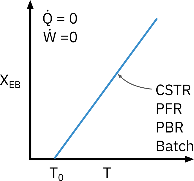
This equation applies to CSTR, PFR, PBR, and Batch reactors. It gives us the explicit relationship between $X$ and $T$ needed to be used in conjunction with the mole balance to solve a large variety of chemical reaction engineering problems.

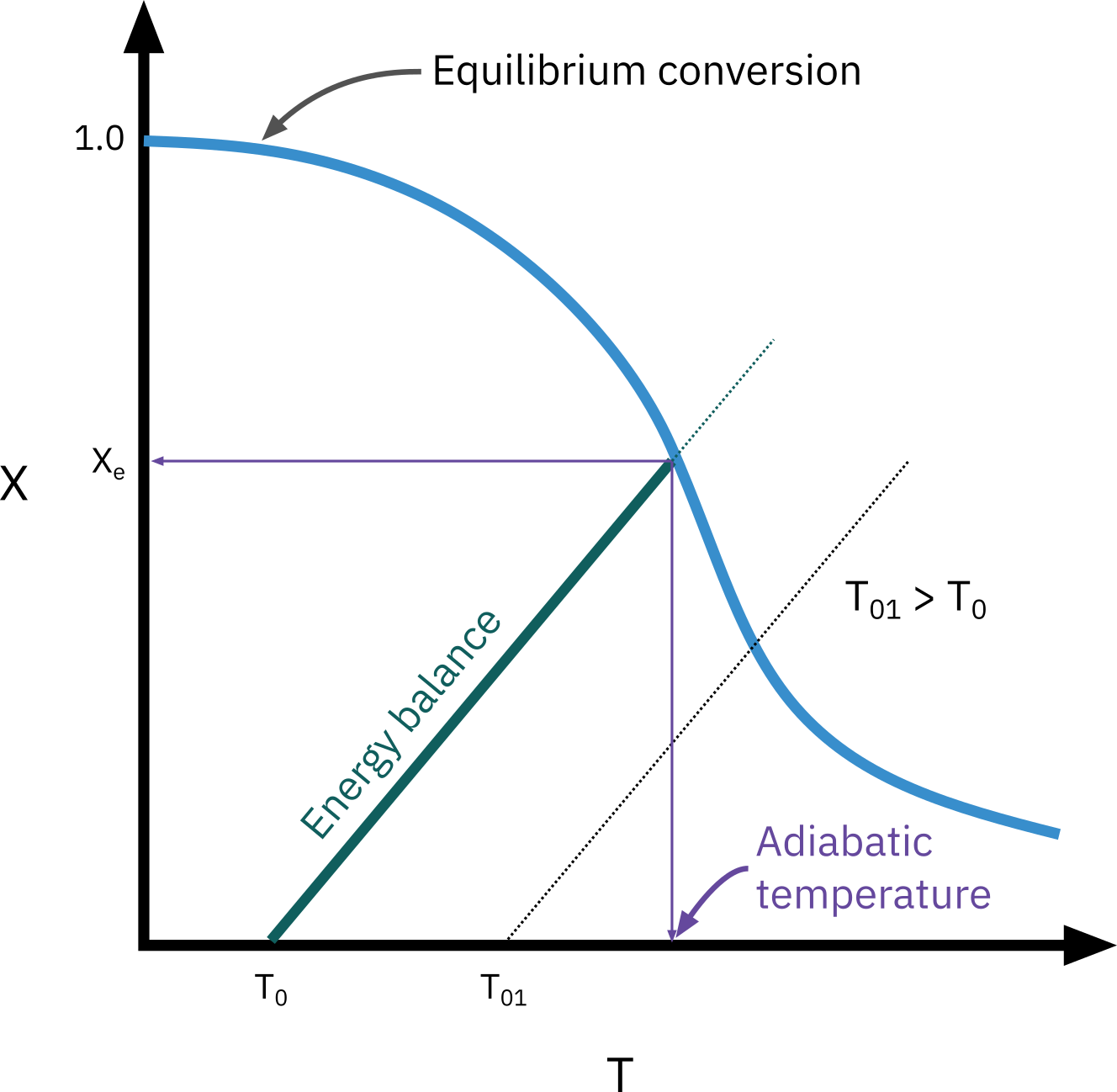
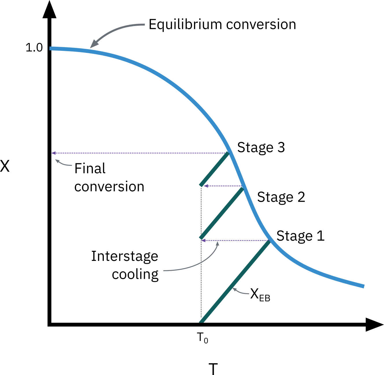
Adiabatic equilibrium conversion

Exothermic reactions

Endothermic reactions

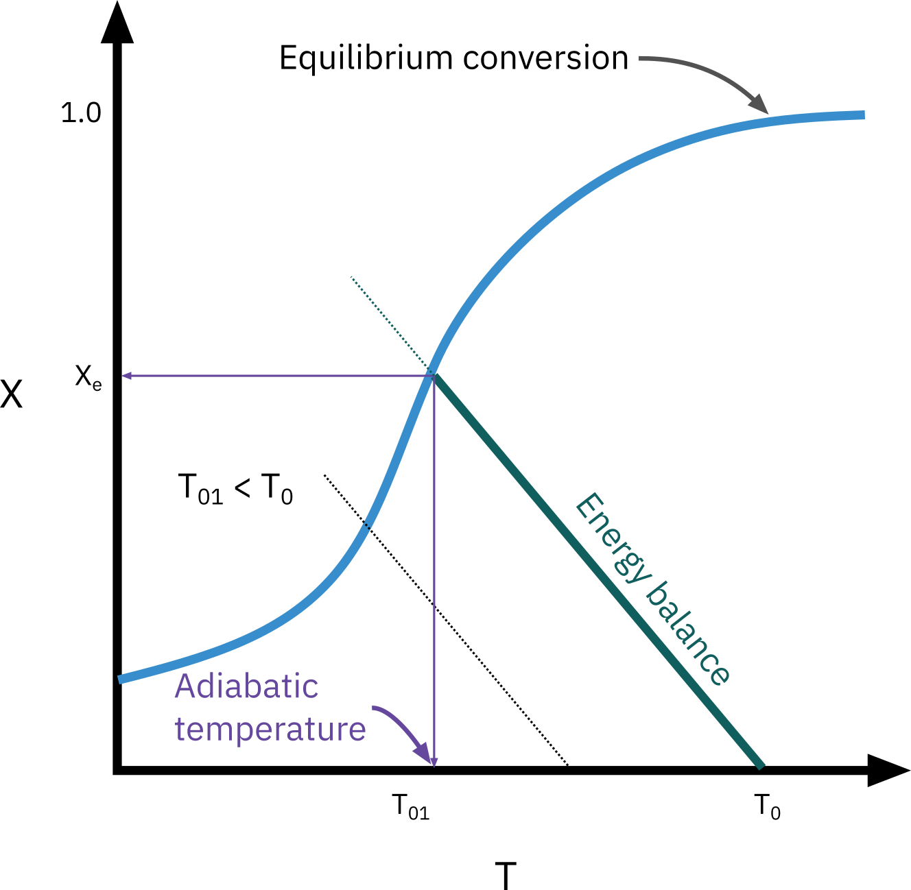
The highest conversion that can be achieved in reversible reactions is the equilibrium conversion. For endothermic reactions, the equilibrium conversion increases with increasing temperature up to a maximum of 1.0. For exothermic reactions, the equilibrium conversion decreases with increasing temperature.

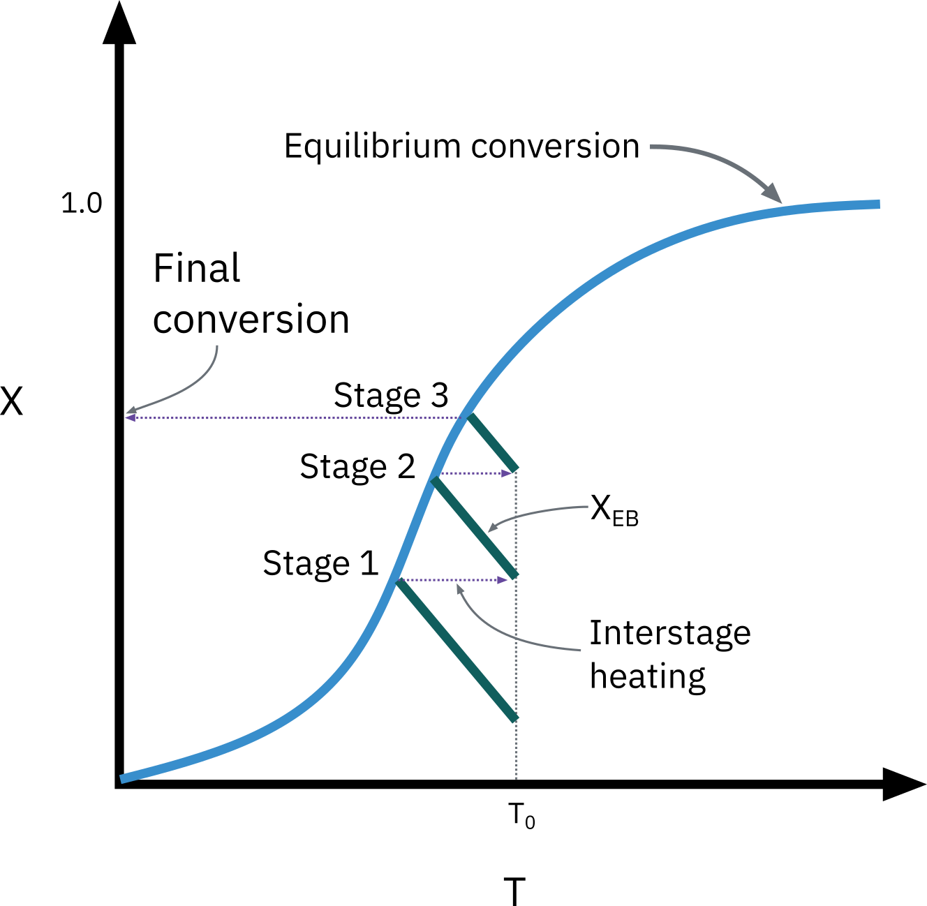
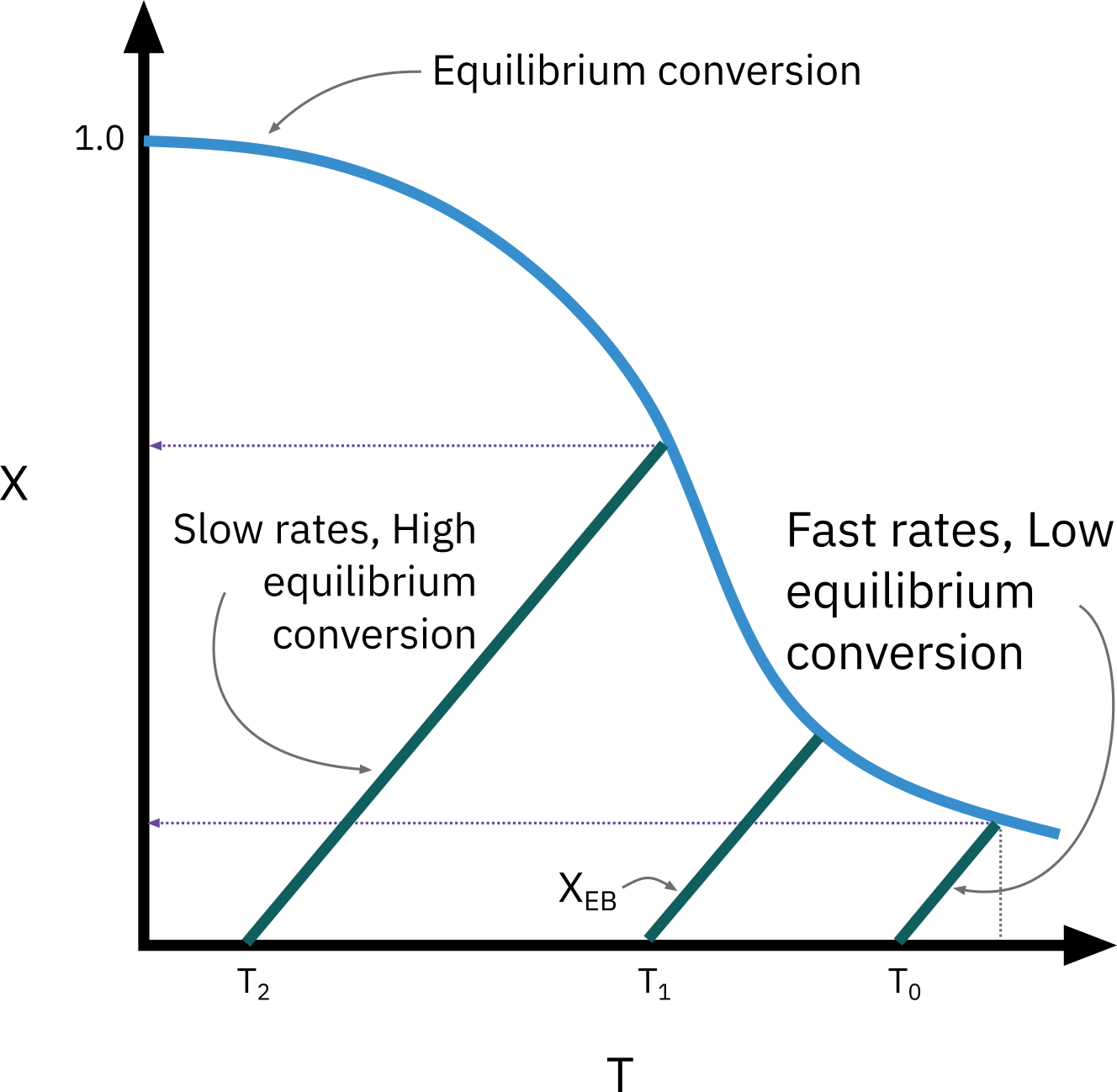
Reactor staging

Exothermic reactions

Endothermic reactions

Optimum feed temperature

Steady-state tubular reactor with heat exchange

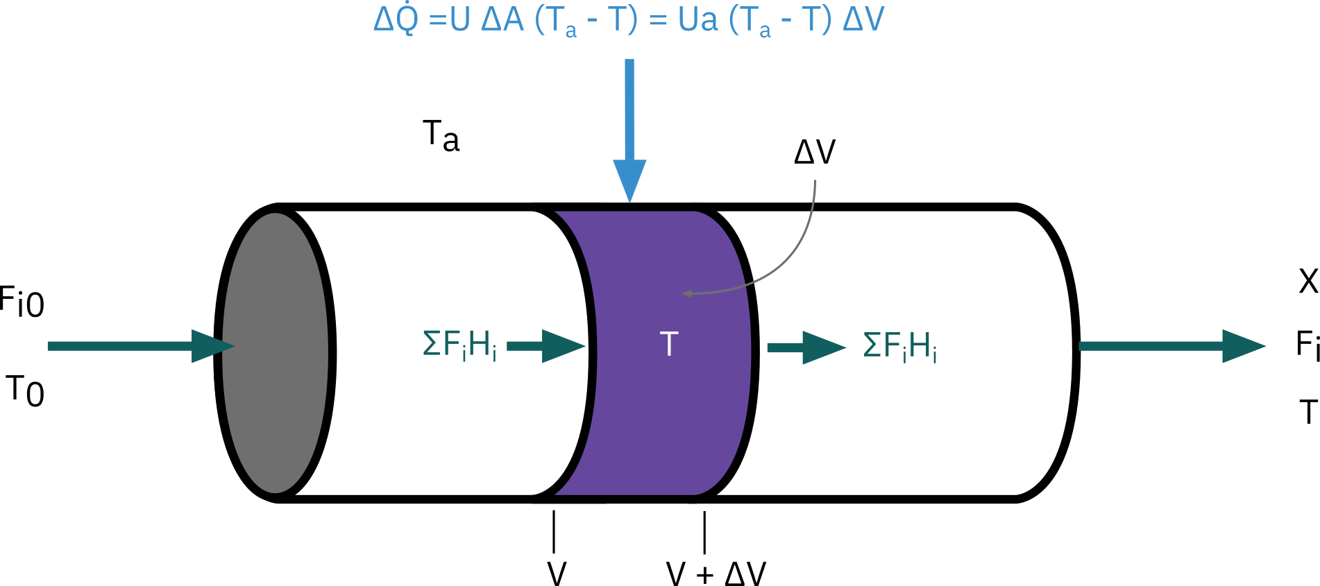
Energy balance over volume $\Delta V$

$\Delta \dot Q + \sum F_i H_i |_V - \sum F_i H_i |_{V + \Delta V} = 0$
Heat flow into the reactor $\Delta \dot Q$

$\Delta \dot Q = U \Delta A (T_a - T) = Ua \Delta V (T_a - T)$

For tubular reactor $a = 4/D$

Dividing by $\Delta V$ and taking limit as $\Delta V \rightarrow 0$

$Ua (T_a - T) - \frac {d\sum F_i H_i}{dV} = 0$

Steady-state tubular reactor with heat exchange

Expanding $Ua (T_a - T) - \sum \frac {dF_i}{dV} H_i - \sum F_i \frac {dH_i}{dV} = 0$
Mole balance: $\frac{dF_i}{dV} = r_i$ also, $\frac{dH_i}{dV} = C_{P_i} \frac{dT}{dV}$

$\frac{dT}{dV} = \frac{ \overbrace{r_A \Delta H_{Rx}(T)}^{\color{black}{\text{Heat generated, } Q_g }} - \overbrace{Ua (T - T_a)}^{\color{black}{\text{Heat removed,} Q_r }} }{ \Sigma_j^{n} F_j C_{P_j} }$

$Q_g = r_A \Delta H_{Rx}(T)$

positive for exothermic reactions; negative for endothermic reactions
When $Q_g > Q_r$ : Temperature will increase as the volume increases
When $Q_g < Q_r$ : Temperature will decrease as the volume increases
For multiple reactions

$Q_g = \sum_i^{n_{rxn}} r_i \Delta H_{Rx,i}(T)$

Balance on the heat-transfer fluid

The heat-transfer fluid will be a coolant for exothermic reactions and a heating medium for endothermic reactions.
If the flow rate of the heat-transfer fluid is sufficiently high with respect to the heat released (or absorbed) by the reacting mixture, then the heat-transfer fluid temperature will be virtually constant along the reactor. For all other cases, we need to write energy balance for the heat transfer fluid.

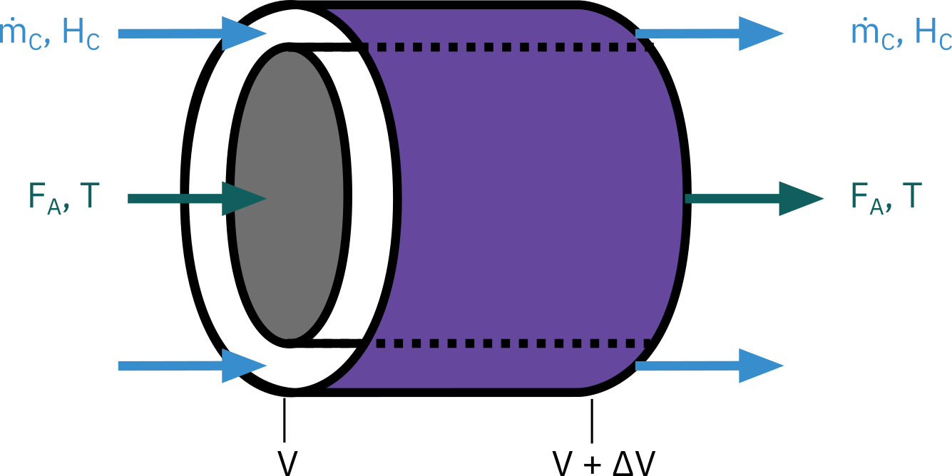
$\begin{aligned} \text{Rate of energy} & & \text{Rate of energy} & & \text{Rate of heat added} & & \\ \text{in at } V & \;\; - & \text{out at } V + \Delta V & \;\; + & \text{by conduction through} & \;\; = & 0 \\ & & & & \text{the inner wall} & & \end{aligned}$

$\dot m_C H_C |_V - \dot m_C H_C |_{ V + \Delta V } + \underbrace{U a (T - T_a) \Delta V}_{\color{RoyalBlue}{\text{Cocurrent flow}}} = 0$

$\frac{dT_a}{dV} = \frac{U a (T - T_a)} { \dot m_C C_{P_C} }$

CSTR with heat effects

Steady state energy balance

$\dot{Q} - \dot{W}_s - F_{A0}\sum \theta_i C_{P,i} (T - T_{i0}) - [\Delta H^{\circ}_{Rx} (T_{Rx}) + \Delta C_{P} (T - T_{Rx})] F_{A0}X = 0$
Shaft work, i.e., the work done by the stirrer or mixer in the CSTR on the reacting fluid inside the CSTR.

As $\dot W_s$ : work done by the system on the surroundings is positive, the CSTR stirrer work will be a negative number.
As $F_{A0} X = -r_A V$

$\dot{Q} - \dot{W}_s - F_{A0}\sum{\theta_i C_{P,i}(T - T_{i0})} + (r_A V)(\Delta H_{Rx}) = 0$

A CSTR’s uniform temperature doesn’t ensure isothermal conditions; for that, the incoming feed must match the reactor’s internal temperature.

Except for processes with highly viscous fluids, the work done by the mixer is typically small enough to ignore.

The $\dot Q$ Term in the CSTR

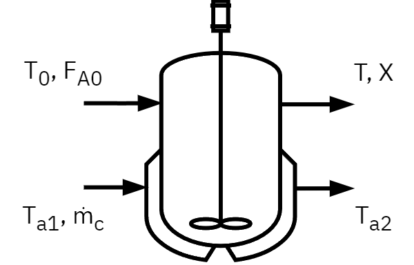
Rate of energy in by flow:

$\dot m_c C_{P,c} (T_{a1} - T_R)$
Rate of energy out by flow:

$\dot m_c C_{P,c} (T_{a2} - T_R)$
Rate of heat transfer from exchanger to reactor:

$\frac{UA(T_{a1} - T_{a2})}{\ln{\left[\frac{(T - T_{a1})} {(T - T_{a2})}\right]}}$

An energy balance on the heat-exchanger fluid entering and leaving the exchanger

$\begin{aligned} \text{Rate of} & & \text{Rate of} & & \text{Rate of} & & \\ \text{energy} &\;\; - & \text{energy} &\;\; - & \text{heat transfer} &\;\; = & \text{0} \\ \text{in} & & \text{out} & & \text{from exchanger} & & \\ \text{by flow} & & \text{by flow} & & \text{to reactor} & & \end{aligned}$

$\dot{Q} = \dot{m}_c C_{P,c} (T_{a1} - T_{a2}) = \frac{UA (T_{a1} - T_{a2})} {\ln\left(\frac{T - T_{a1}}{T - T_{a2}}\right)}$

$T_{a2} = T - (T - T_{a1}) \exp \left( \frac{-UA}{\dot{m}_c C_{P,c}} \right)$

$\dot{Q} = \dot{m}_c C_{P,c} \left( T_{a1} - T \right) \left[ 1 - \exp \left( \frac{-UA}{\dot{m}_c C_{P,c}} \right) \right]$

For very large $\dot m_c$

$\dot{Q} = U A (T_a - T)$

Conversion in a non-adiabatic CSTR

Ignoring $\dot W_s$

$\frac{UA}{F_{A0}} (T_a - T) - \sum \theta_i C_{P,i} (T - T_0) - \Delta H^{\circ}_{Rx} X = 0$
Solving for $X$

$X = \frac{\frac{UA}{F_{A0}} (T - T_a) + \sum \theta_i C_{P,i} (T - T_0)} {-\Delta H^{\circ}_{Rx} (T_R)} \tag{1}$
Couple Equation 1 with the mole balance equation $V = \frac{F_{A0}X}{-r_A (X, T)}$ to design CSTR
Rearranging

$X = \frac{C_{P,o} (1 + \kappa) (T - T_c)}{-\Delta H^{\circ}_{Rx}} \quad \text{and} \quad T = T_c + \frac{(-\Delta H^{\circ}_{Rx})(X)}{C_{P,o}(1 + \kappa)}$

$\text{Where} \quad C_{P,o} = \sum \theta_i C_{P,i} \quad \text{,} \quad \kappa = \frac{UA}{F_{A0} C_{P,o}} \quad \text{,and} \quad T_c = \frac{\kappa T_a + T_0}{1 + \kappa}$