Collection and analysis of rate data
Chemical Reaction Engineering
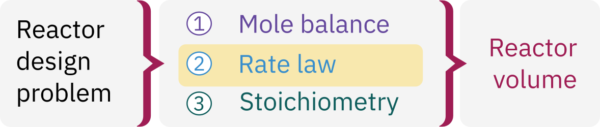
Isothermal reactor design algorithm
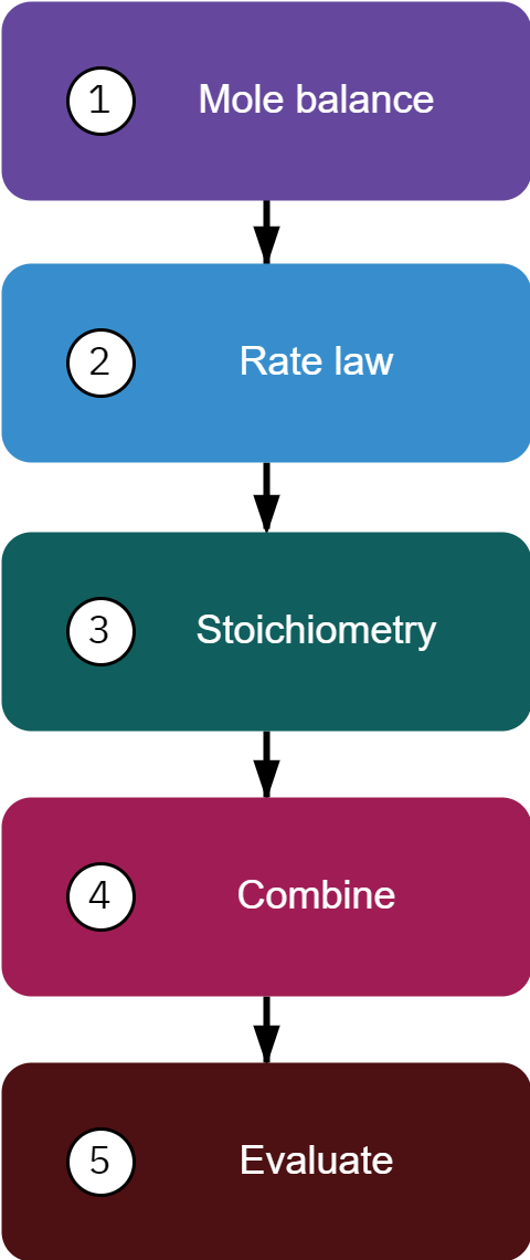
Mole balance
F_{A0} - F_A = \int^V r_A dV = \frac{dN_A}{dt}
Rate law
If -r_A is given as f(X) \rightarrow directly solve the design equations
Stoichiometry
If -r_A = g(C) \rightarrow use stoichiometry to write -r_A = f(X)
Combine
Gather all equations to obtain a system of equations that must be solved.
Evaluate
The system of equation scan be solved analytically, graphically, numerically, or using software
Isothermal reactions in PBR: molar flow rates
Second order reaction \ce{aA + bB -> cC + dD}
Mole balance: Write balance for each species i = 1 \ to \ N
\frac{dF_i}{dW} = r'_i
Rate law
-r'_A = kC_A^\alpha C_B^\beta; \qquad \frac{r'_A}{-a} = \frac{r'_B}{-b} = \frac{r'_C}{c} = \frac{r'_D}{d}
Stoichiometry C_i = \frac{C_{A0} (\Theta_i + \nu_i X)} {(1 + \epsilon X)} \left( \frac{P}{P_0} \right) \left( \frac{T_0}{T} \right)
Pressure: \frac{dP}{dW} = -\frac{\alpha}{2p} \left( \frac{T}{T_0} \right) \frac{F_T}{F_{T0}}
Total molar flow rate: F_T = \sum_{i=1}^N F_i
Combine:
Collate all equations from steps 1 to 3 to yield a system of equations
Evaluate:
Use ODE solver to solve the system of equations obtained in step 4.
Reactor design problem
![]()
In practice, collection and analysis of rate data is the most time consuming task in reactor design
![]()
Data collection is done in the lab, where we can simplify mole balance, stoichiometry, and fluid dynamic considerations
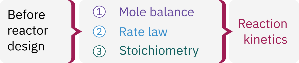
Algorithm for rate data analysis
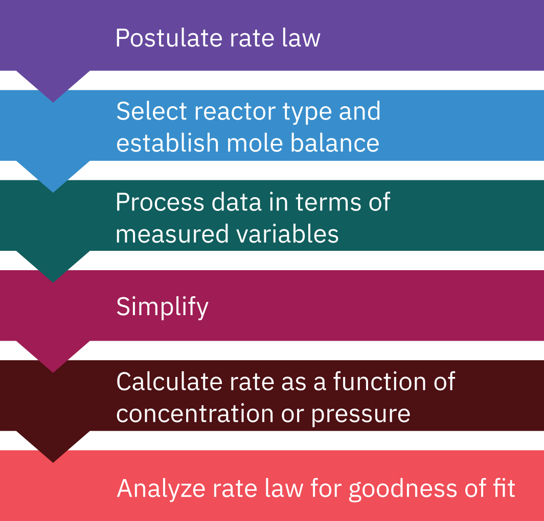
Determination of rate law for homogenous reactions
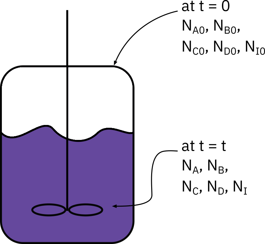
Most often batch reactors are used
Type of reactor chosen will not affect rate of reaction
Batch reactor
- Simple operations, low cost
- Ease of sampling, easy clean up, limited waste
- Uniform concentration can be obtained
Mole balance: constant volume -\frac{dC_A}{dt} = -r_A
- Typical measurements
- Concentration Pressure
- Temperature: Many times batch reactions are carried out isothermally.
- Development of heat during reaction: Reaction calorimetry
Method of excess
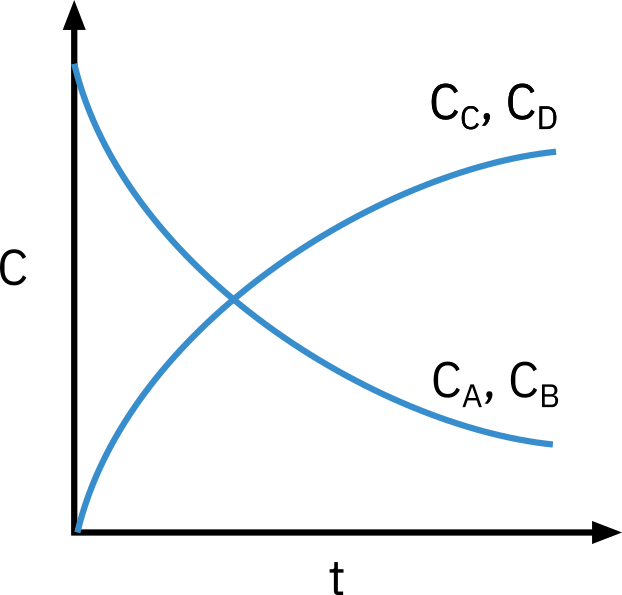
Given concentration vs. time profile in a batch experiment, determine the reaction order and rate constant.
\ce{A + B -> C + D}
- Rate law: -r_A = k C_A^\alpha C_B^\beta
- Need to determine: k, \alpha, and \beta
Determining reaction orders: \alpha, and \beta
Common simplification: One of the reactants is in excess
Two separarate experiments
Excess B \Rightarrow C_B \gg C_A, C_B can be assumed constant. \Rightarrow determine \alpha.
Excess A \Rightarrow C_A \gg C_B, C_A can be assumed constant. \Rightarrow determine \beta.
Determining k: Measuring rate at known concentrations of A, and B.
Differential analysis
Irreversible reaction
The rate is essentially a function of the concentration of only one reactant.
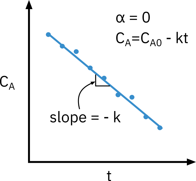
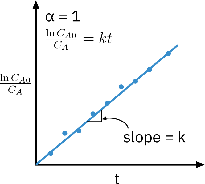
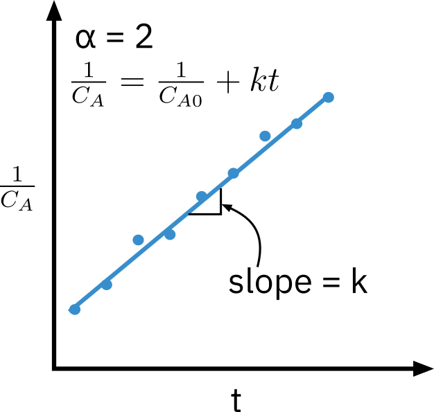
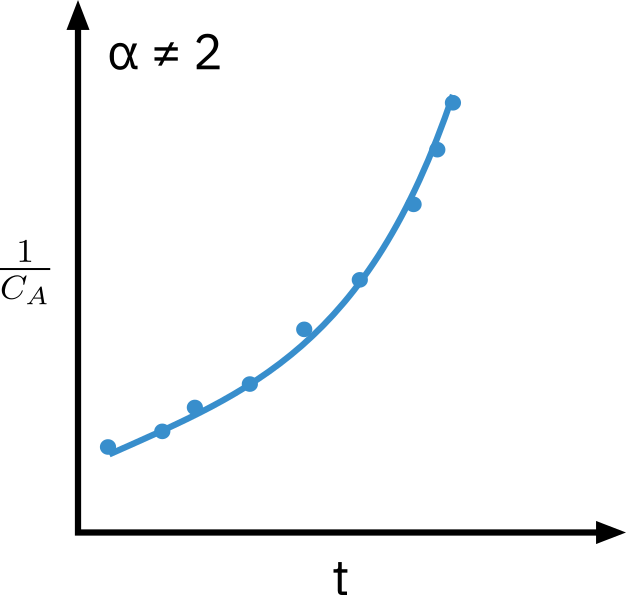
\ce{A -> products}; -r_A = k C_A^\alpha
Isothermal, constant volume batch reactor
Mole balance: constant volume -\frac{dC_A}{dt} = -r_A; -r_A = k C_A^\alpha
Taking natural logarithm
\ln \left( \frac{-dC_A}{dt} \right) = \ln k + \alpha \ln C_A
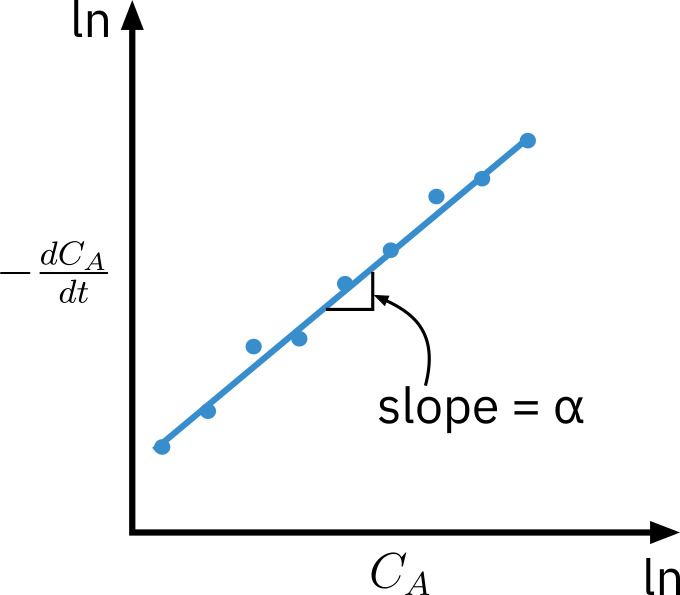
Slope of plot of \ln[ -dC_A/dt ] \ \text{vs.} \ln C_A is the reaction order
Specific reaction rate can be determined using a specific point p: k = \frac{(-dC_A/dt)_p}{(C_A)_p^\alpha}
Evaluating \frac{-dC_A}{dt}
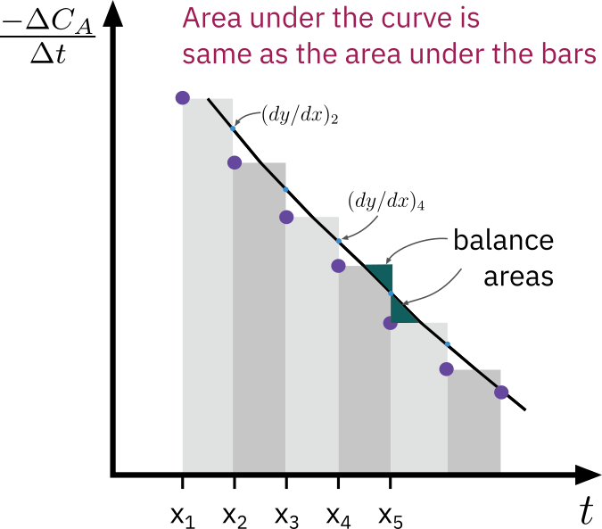
Graphical diffrentiation
- Very old method
- Equal area graphical diffrentiation
- Disparities in the data are easily seen
Numerical diffrentiation
- Finite difference
- Independent variable (time) is equally spaced
Diffrentiation of a polynomial fit to the data
Fit a polynomial to C_A \ \text{vs.} \ t data
e.g. C_A = f(t) = a_0 + a_1 t + a_2 t^2 + a_3 t^3 + a_4 t^4
Analytical derivative
\frac{dC_A}{dt} = f'(t) = a_1 + a_2 t + a_3 t^2 + a_4 t^3
- Determine reaction order and specific rate from plot of \ln[ -dC_A/dt ] \ \text{vs.} \ln C_A
Integral analysis
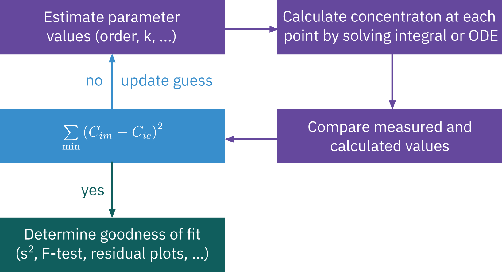
Nonlinear regression
Search for parameter values that minimize the sum of squares of the difference between the measured values and calculated values for all data points.
Best estimate of parameter values
Discriminate between different rate law models
Godness of fit
Root Mean Squared Error (RMSE) and Mean Absolute Error (MAE)
Lower values indicate a better fit. RMSE is sensitive to outliers, while MAE provides a more robust error metric.
P-value of the F-test in ANOVA (Analysis of Variance)
A p-value smaller than the significance level (commonly 0.05) indicates that there is a statistically significant relationship.
Residual Plots
Ideally, the residuals should be randomly scattered around 0 across the range of fitted values. Patterns in the residual plot can indicate problems with the model
Method of half life
t_{1/2} = \frac{1}{k C_{A0}^{\alpha -1} (\alpha -1)} \left[ 2^{\alpha -1} -1 \right]
Taking log
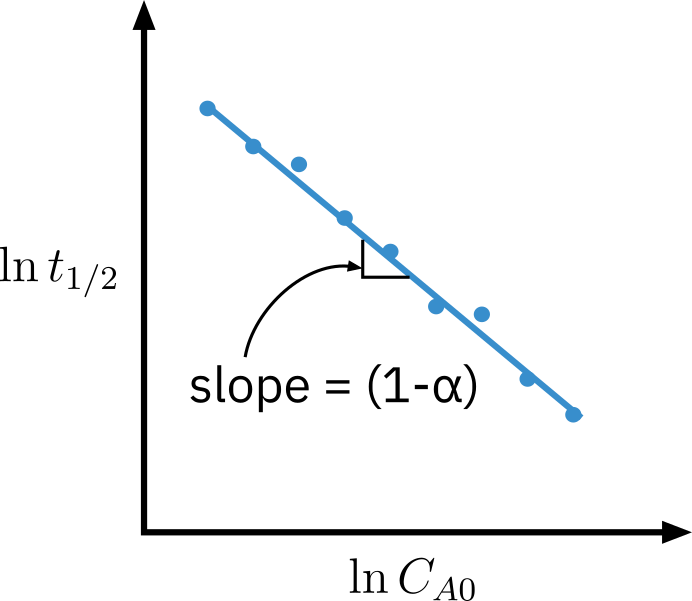
\ln t_{1/2} = \ln \frac{2^{\alpha - 1} - 1}{(\alpha -1) k} + (1-\alpha) \ln C_{A0}
Multiple experiments are performed varying initial concentration and t_{1/2} is recorded.
The plot of \ln t_{1/2} vs. \ln C_{A0} is linear with a slope of (1 - \alpha)
Method of initial rates
Perform a series of experiments at different initial concentrations C_{A0}
Determine initial rate of reaction -r_{A0}
Determine rate law parameters by relating -r_{A0} to C_{A0}
Reaction: \ce{A -> products}
Rate law: -r_A = k C_A^\alpha
Mole balance: -\frac{dC_A}{dt} = k C_A^\alpha
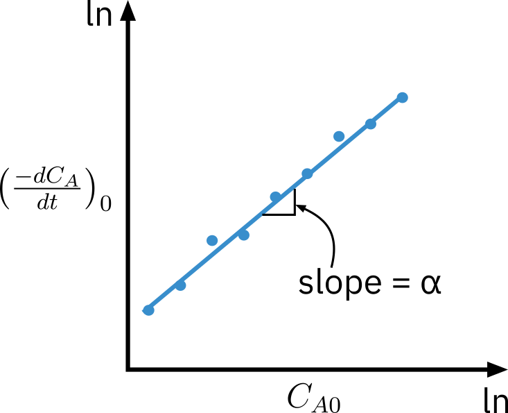
Initial rate: -r_{A0} = \left( \frac{-dC_A}{dt}\right)_0 = k C_{A0}^\alpha
- Taking log
\ln \left( \frac{-dC_A}{dt}\right)_0 = \ln k + \alpha \ln C_{A0}
Rate data from differential reactors
For heterogeneous reactions mostly packed bed reactors (PBRs) are used.
Differential reactor: The conversion of the reactants in the bed is extremely small, as is the change in reactant concentration through the bed
Reactant concentration through the reactor is essentially constant (i.e. the reactor is considered to be gradient-less)
Can treat the mole balance like a CSTR
Rate of reaction determined for a specified number of pre-determined initial or entering reactant concentrations
Determine rate of reaction as a function concentration or partial pressure
Operate isothermally
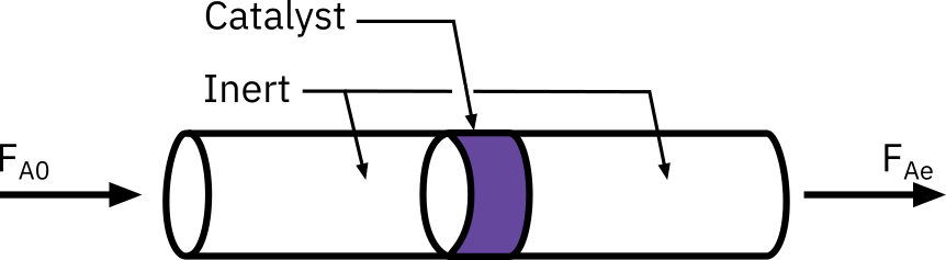
Differential reactor
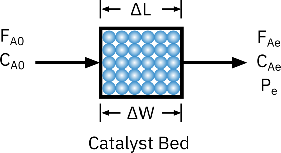
Assumptions
- No concentration and temperature gradient (gradientless reactor)
- High volumetric flow rate
- Small catalyst particles (No mass transfer limitation)
- Very low conversion
- Low/ negligible heat release (isothermal)
- No bypassing/ channeling (uniform flow across catalyst layer)
Mole balance:
in - out + generation = accumulation
F_{A0} - F_{Ae} + r'_A \Delta W = 0
-r'_A = \frac{F_{A0} - F_{Ae}}{\Delta W} = \frac{\upsilon_0 C_{A0} - \upsilon C_{Ae}}{\Delta W}
- For constant flow rate \upsilon = \upsilon_0
-r'_A = \frac{\upsilon_0 C_{A0} X}{\Delta W} = \frac{\upsilon_0 C_{P}}{\Delta W}
\rightarrow For small conversion -r'_A can be expressed as a function of C_{A0}