Conversion and reactor sizing

Chemical Reaction Engineering

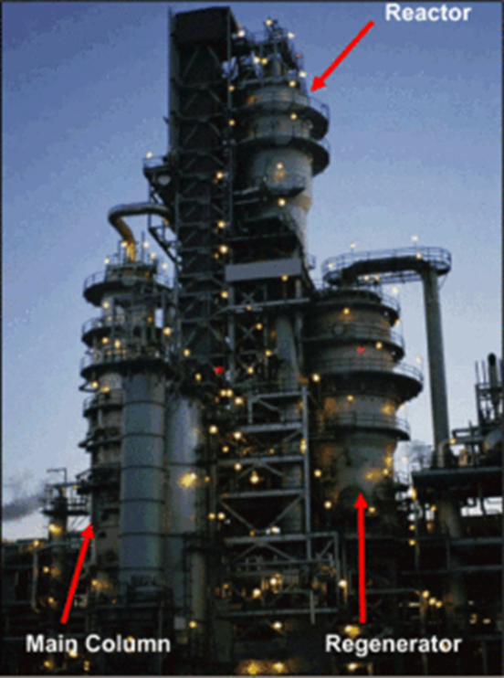
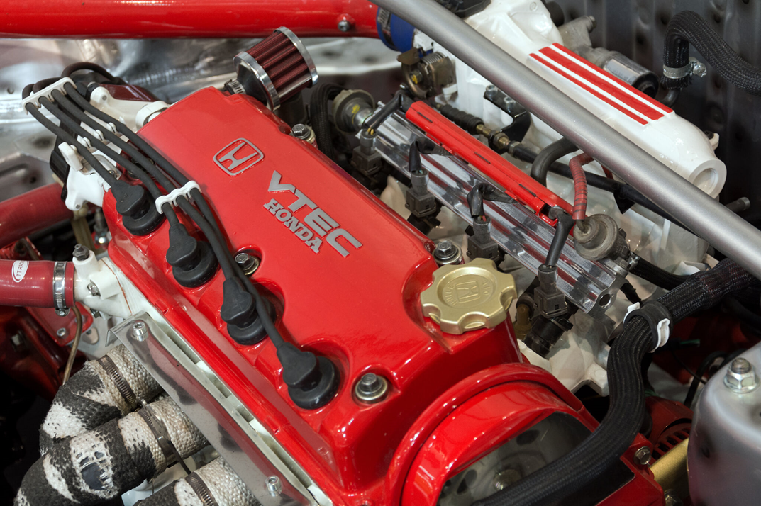
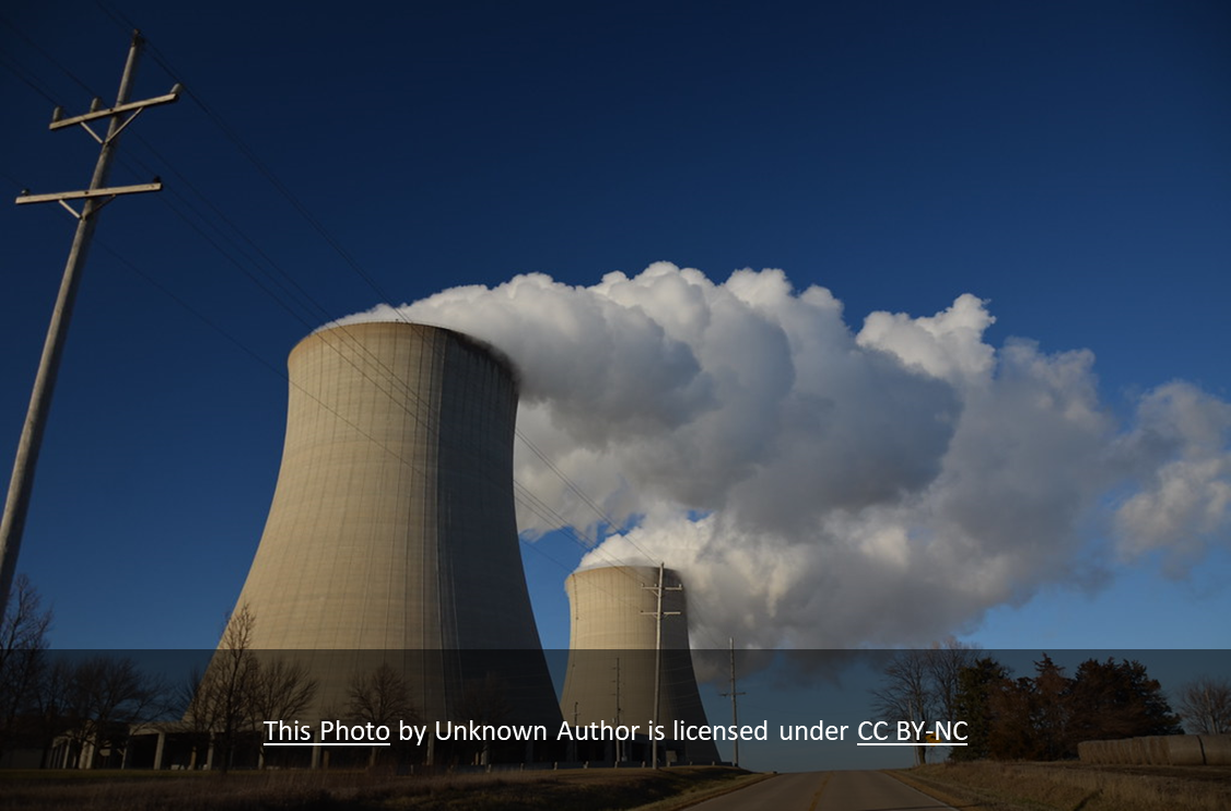
Is this a reactor

Review - general mole balance

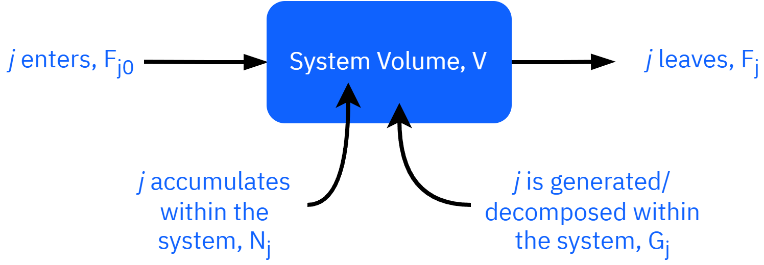
General form: F_{j0} - F_j + G_j = \frac{dN_j}{dt}
Uniform generation F_{j0} - F_j + r_j V = \frac{dN_j}{dt}
Non-uniform generation F_{j0} - F_j + \int^V r_j dV = \frac{dN_j}{dt}

Reactor mole balance

Reactor	Differential form	Algebraic form	Integral form
Batch	\frac{dN_A}{dt} = r_AV		t = \int_{N_{A0}}^{N_A} \frac{dN_A}{r_A V}
CSTR		V = \frac{F_{A0} - F_A}{-r_A}
PFR	\frac{dF_A}{dV} = r_A		V = \int_{F_{A0}}^{F_A} \frac{dF_A}{r_A}
PBR	\frac{dF_A}{dW} = r'_A		W = \int_{F_{A0}}^{F_A} \frac{dN_A}{r'_A}

Conversion, X

Conversion is convenient for relating: r_j, V, \upsilon, N_j, F_j, \text{and } C_j
Consider the generic reaction

\ce{a A + b B -> c C + d D}
Choose limiting reactant A as basis of calculation and normalize

\ce{ A + \frac{b}{a} B -> \frac{c}{a} C + \frac{d}{a} D}
Conversion (X): The fraction or percentage of a reactant that is consumed during a chemical reaction.

X = \frac{\text{moles of A reacted}}{\text{moles of A fed}}
Batch system: “Moles A fed” is the amount of A at the start of the reactor (t=0) Flow system: “Moles A fed” is the amount of A entering the reactor

Conversion, X

Consider \ce{A + 2B -> 2C}, Start with 1 mole of A, and 1 mole of B

A is the basis:

At the end we have

1 mole A, 1 mole B

X_A = 0/1 = 0 \Rightarrow \text{no reaction}
\frac{1}{2} mole A, 0 mole B

X_A = 0.5/1 = 1/2 (0.5)
0 mole A, -1 mole B

X_A = 1/1 = 1 \Rightarrow \text{complete reaction, but not possible}

B is the basis:

At the end we have

1 mole A, 1 mole B

X_B = 0/1 = 0 \Rightarrow \text{no reaction}
\frac{1}{2} mole A, 0 mole B

X_B = 1/1 = 1 \Rightarrow \text{complete reaction}

Pick the limiting reagent as the basis to calculate conversion

Moles and molar flow rate in terms of X_A

\ce{ A + \frac{b}{a} B -> \frac{c}{a} C + \frac{d}{a} D} \qquad \qquad X = \frac{\text{moles of A reacted}}{\text{moles of A fed}}

Batch systems: Longer reactant is in reactor, more reactant is converted to product (until reactant is consumed or the reaction reaches equilibrium)

N_A = N_{A0} - N_{A0} X_A

N_A = N_{A0}( 1 - X_A)
Flow systems: For a given flow rate, the larger the reactor, the more time it takes the reactant to pass through the reactor, the more time to react

F_A = F_{A0} - F_{A0} X_A

F_A = F_{A0}( 1 - X_A)

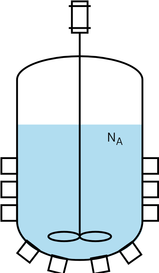
Design equation in terms of X: Batch reactor

Ideal batch reactor design equation

\frac{dN_A}{dt}=r_A V
N_A = N_{A0}( 1 - X_A)
Taking the derivative of N_A equation

\frac{d}{dt}N_A = \frac{d}{dt}\left( N_{A0}(1 - X_A)\right)

\frac{dN_A}{dt} = 0 - N_{A0}\frac{dX_A}{dt}
Substituting

N_{A0} \frac{dX_A}{dt} = -r_A V

t = N_{A0} \int_0^{X_A}\frac{dX_A}{-r_A V}

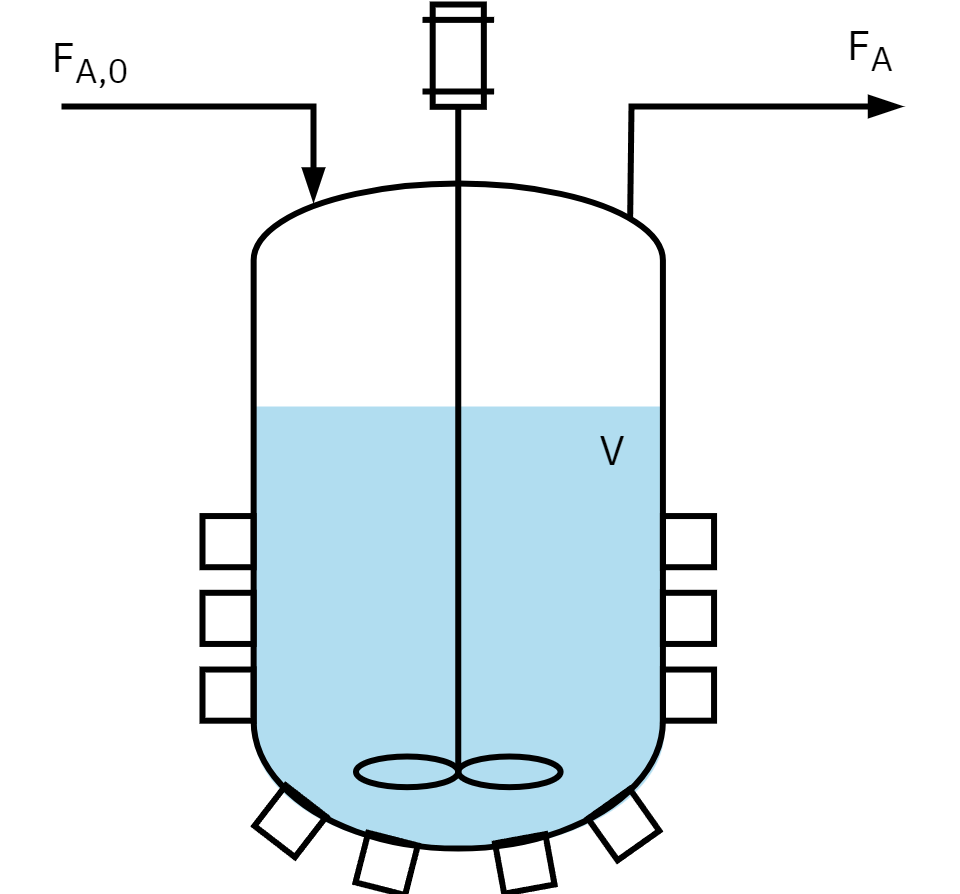
Design equation in terms of X: CSTR

Ideal steady state CSTR design equation

V = \frac{F_{A0}-F_A}{-r_A}
Substitute for F_A

F_A = F_{A0}( 1 - X_A)

V = \frac{\cancel{F_{A0}} - \left[ \cancel{F_{A0}} - F_{A0} X_A \right]}{-r_A}
V = \frac{F_{A0} X_A}{-r_A}

V is the CSTR volume required to achieve a specified conversion. X_A and –r_A are evaluated at the exit of the CSTR

Design equation in terms of X: PFR

Ideal steady state PFR design equation

\frac{dF_A}{dV} =r_A
F_A = F_{A0}( 1 - X_A)
Taking the derivative of F_A equation

\frac{d}{dV}F_A = \frac{d}{dV}\left( F_{A0}(1 - X_A)\right)

\frac{dF_A}{dV} = 0 - F_{A0}\frac{dX_A}{dV} \qquad \Rightarrow \qquad \frac{dF_A}{dV} = - F_{A0}\frac{dX_A}{dV}
Substituting

F_{A0} \frac{dX_A}{dV} = -r_A \qquad \Rightarrow \qquad V = F_{A0} \int_0^{X_A} \frac{dX_A}{-r_A}

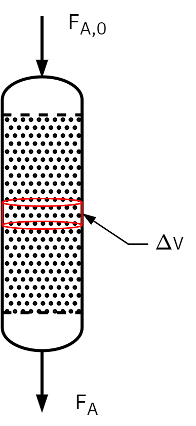
Design equation in terms of X: PBR

Ideal steady state PBR design equation

\frac{dF_A}{dW} =r'_A
F_A = F_{A0}( 1 - X_A)
Taking the derivative of F_A equation

\frac{d}{dW}F_A = \frac{d}{dW}\left( F_{A0}(1 - X_A)\right)

\frac{dF_A}{dW} = - F_{A0}\frac{dX_A}{dW}
Substituting

F_{A0} \frac{dX_A}{dW} = -r'_A \Rightarrow W = F_{A0} \int_0^{X_A} \frac{dX_A}{-r'_A}

::::

Reactor mole balance in terms of X

Reactor	Differential form	Algebraic form	Integral form
Batch	N_{A0}\frac{dX}{dt} = r_AV		t = N_{A0}\int_0^{X} \frac{dX}{r_A V}
CSTR		V = \frac{F_{A0}X}{-r_A}
PFR	F_{A0}\frac{dX}{dV} = -r_A		V = F_{A0} \int_{0}^{X} \frac{dX}{-r_A}
PBR	F_{A0}\frac{dX}{dW} = -r'_A		W = F_{A0} \int_{0}^{X} \frac{dX}{-r'_A}

Sizing of continuous flow reactors

Sizing refers to either of
- Determining reactor volume for specified conversion
- Determining conversion for a specified volume
For All irreversible reactions of order greater than 0, As we approach complete conversion, the reciprocal rate approaches infinity

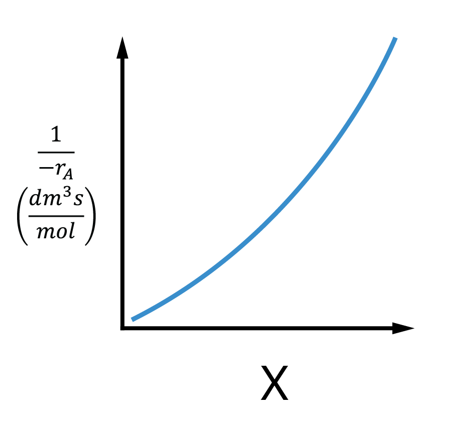
Irreversible reaction:

As X \rightarrow 1 ; -r_A \rightarrow 0
Reversible reaction:

As X \rightarrow X_e ; -r_A \rightarrow 0

\Rightarrow \frac{1}{-r_A} \rightarrow \infty \therefore V \rightarrow \infty

Infinite reactor volume is necessary to reach complete conversion

Sizing of continuous flow reactors

CSTR

V = \left( \frac{F_{A0}}{(-r_A)_{exit}} \right) \cdot X

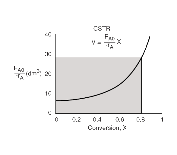
CSTR volume

area of rectangle bound by X_A and \frac{F_{A0}}{-r_{A, exit}}

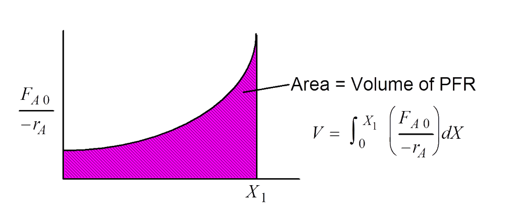
PFR

V = \int_0^X \left( \frac{F_{A0}}{(-r_A)}\right) dX

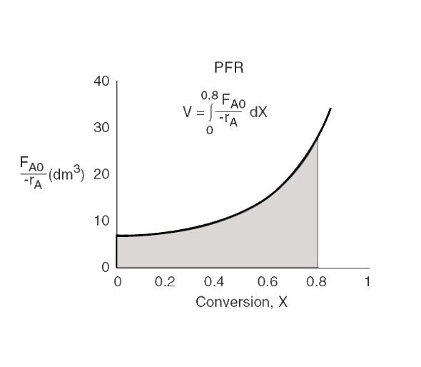
PFR volume

area under the curve \frac{F_{A0}}{-r_{A}} = f(X_A)

Levenspiel plots - reactor sizing

Given –r_A as a function of conversion, -r_A= f(X), one can size any type of reactor.
We do this by constructing a Levenspiel plot.
Here we plot either \frac{F_{A0}}{-r_A} or \frac{1}{-r_A} as a function of X.

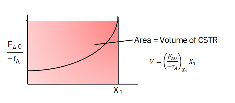
CSTR sizing

Using following data: Calculate V_{CSTR} for X = 0.4, and X = 0.8

X	0.00	0.10	0.20	0.40	0.60	0.70	0.80
\frac{F_{A0}}{-r_A}	0.89	1.08	1.33	2.05	3.56	5.06	8.00

V = \left( \frac{F_{A0}}{(-r_A)_{exit}} \right) \cdot X

For X = 0.4; \frac{F_{A0}}{(-r_A)_{exit}} = 2.05 m^3

V = 0.82 m^3
For X = 0.8; \frac{F_{A0}}{(-r_A)_{exit}} = 8.00 m^3

V = 6.4 m^3

PFR sizing

Using following data: Calculate V_{PFR} for X = 0.4, and X = 0.8

X	0.00	0.10	0.20	0.40	0.60	0.70	0.80
\frac{F_{A0}}{-r_A}	0.89	1.08	1.33	2.05	3.56	5.06	8.00

V = \int_0^X \left( \frac{F_{A0}}{(-r_A)}\right) dX

For X = 0.4; Numerically integrate the data

V = 0.55 m^3
For X = 0.8; \frac{F_{A0}}{(-r_A)_{exit}} = 8.00 m^3

V = 2.15 m^3

Reactors in series

Reactors are arranged sequentially, with the output of one reactor feeding directly into the next.
Advantages:
- Achieve higher overall conversion rates
- Handle reactions requiring different conditions at different stages.
- Different reaction conditions can be optimized in each reactor.
- Staging: Allows for the introduction of intermediates or the removal of by-products between stages.
Both Continuous Stirred Tank Reactors (CSTRs) and Plug Flow Reactors (PFRs) can be configured in series, either separately or in a mixed arrangement, to optimize reaction conditions and efficiencies.
Key Considerations
- Reactor volume and design optimization
- Maintenance and operational complexity

Levenspiel plots can be used to visualize and sequence reactors in series.

Reactors in series

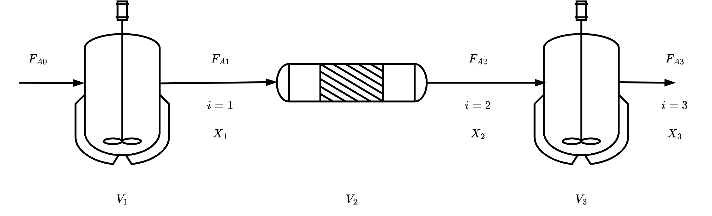
In absence of any side streams (inlets or outlets)

Conversion up to point i:

X_i = \frac{\text{total moles of A reacted up to point } i }{\text{Moles A fed into } 1^{st} \text{ reactor}}
Molar Flow rate of species A at point i:

F_{Ai} = F_{A0} - F_{A0} X_i

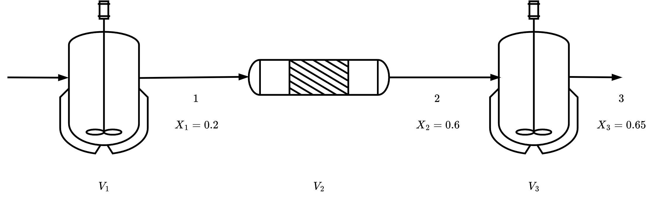
Reactors in series

Example: An adiabatic liquid-phase isomerization

The isomerization of butane

\ce{n-C4H10 <=> i-C4H10}

was carried out adiabatically in the liquid phase. The data for this reversible reaction are given below. Calculate the volume of each of the reactors for an entering molar flow rate of n-butane of 50 kmol/hr.

X	0.00	0.20	0.40	0.60	0.65
-r_A, \frac{kmol}{m^3 \cdot h}	39.00	53.00	59.00	38.00	25.00

Reactors in series

Example: An adiabatic liquid-phase isomerization

Reactors in series

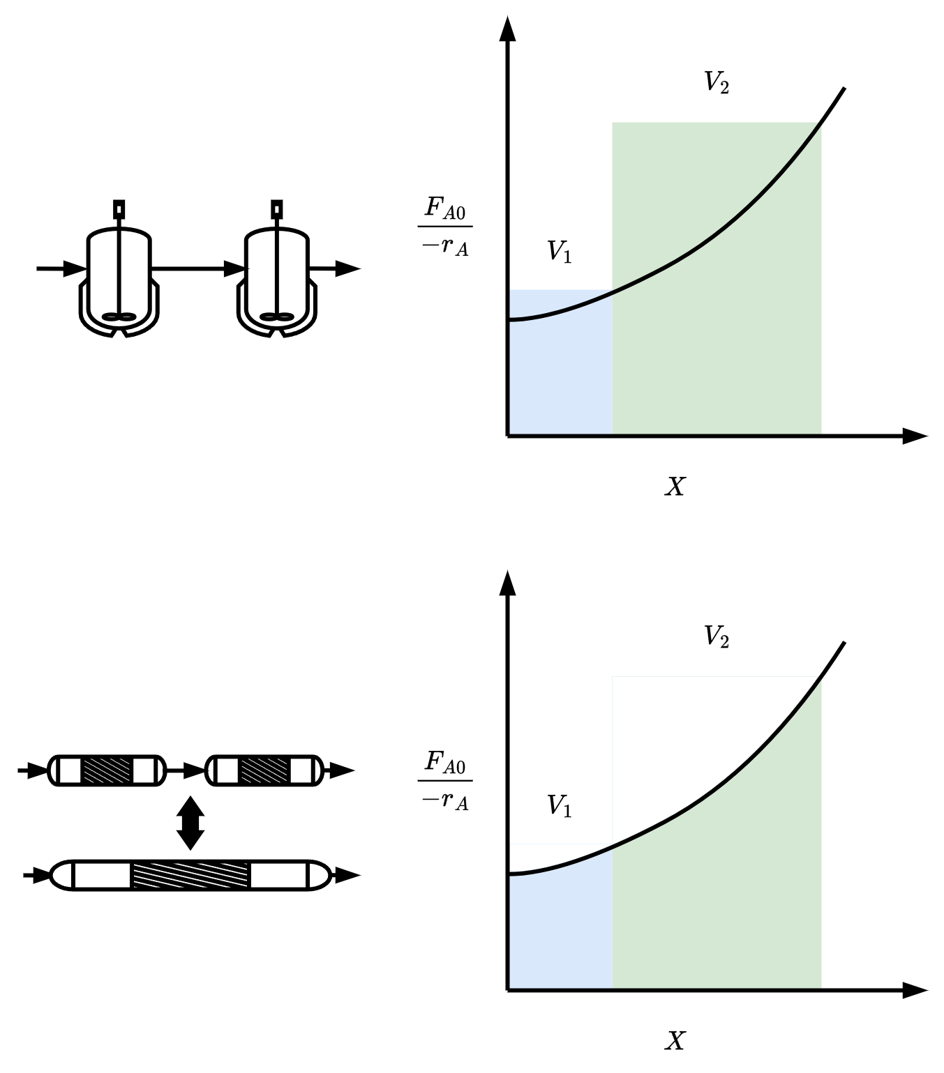
If \frac{F_{A0}}{-r_A} monotonically increases with X

V_{\text{one PFR}} \leq \sum_i V_{\text{PFR(i)}} + \sum_j V_{\text{CSTR(j)}} \leq V_{\text{one CSTR}}

for any combination of PFRs and CSTRs in series

In general

1 PFR = any number of PFRs in series

1 PFR = \infty number of CSTRs in series
For large number of CSTRs in series, the total volume is ‘roughly’ same as volume of PFR

The concept of using CSTRs in series to model PFR is used in larger number of situations such as modeling catalyst decay in packed bed reactors, or studying transient heat effects in PFR.

Space time (\tau)

Time necessary to process one reactor volume, also called mean residence time or holding time

\tau = \frac{V}{\upsilon_0}
Space velocity (SV): inverse of space time, but vo may be measured under different conditions than the space time

SV = \frac{\upsilon_0}{V} = \frac{1}{\tau}
- LHSV: Liquid hourly space velocity: \mathrm{LHSV} =\frac{\upsilon_{0 \mid \mathrm{liquid}}}{V}
- GHSV: Gas hourly space velocity: \mathrm{GHSV}=\frac{\upsilon_{0 \mid \mathrm{STP}}}{V}
- \upsilon_{0 \mid} is the volumetric flow rate measured at specified condition